flowchart LR
    subgraph Corporate
        A1[Estimate PD] --> D1[Risk-weight function]
        B1[Estimate LGD] --> D1
        C1[Estimate EAD] --> D1
        D1 --> E1[RWA Corporate]
        style A1 fill:#ddeaf1,stroke:#333,stroke-width:2px
        style B1 fill:#ddeaf1,stroke:#333,stroke-width:2px
        style C1 fill:#ddeaf1,stroke:#333,stroke-width:2px
    end
    subgraph Sovereign
        A2[...] -->
        E2[RWA Sovereign]
    end
    subgraph Financial Institution
        A3[...] --> E3[RWA Financial]
    end
    subgraph Retail
        A4[...] --> E4[RWA Retail]
    end
    E1 --> F[Aggregation]
    E2 --> F
    E3 --> F
    E4 --> F
    F --> G[Total Credit Risk RWA]
AFIN8003 Week 7 Workshop - Credit Risk Modelling in Practice
Banking and Financial Intermediation
AFIN8003
2026S2
Credit Risk Modelling in Practice
Why this workshop exists
- Week 6 measured credit risk on an individual loan.
- Week 7 lecture covered the portfolio view (concentration, migration, CDS).
- This workshop fills in the practical middle: how a bank actually estimates PD, calibrates it, and turns it into regulatory capital using the Internal Ratings-Based (IRB) model.
Every piece in this deck is a building block you will find useful in the group assignment. By the end of the session you should be able to look at a loan book and reason about regulatory capital end-to-end.
Roadmap: 8 widgets, 9 parts
- IRB three parameters (PD, LGD, EAD)
- Widget 1: IRB RWA calculator
- Building a PD model: data and pipeline
- Widget 2: Information Value intuition
- Widget 3: Logistic curve visualiser · Widget 4: ROC and threshold slider
- Widget 5: Rating bin tuner (calibration)
- Widget 6: Transition matrix heatmap (validation)
- Widgets 7–8: Altman Z-score · Merton distance-to-default
- Knowledge check + wrap-up
Everything runs in your browser. Nothing to install. Nothing to download. Slide numbers are in the footer, so if you get lost, shout a number.
Credit risk dominates the capital stack
| CBA | Westpac | NAB | ANZ | Macquarie | |
|---|---|---|---|---|---|
| RWA for credit risk | 370,444 | 351,724 | 350,891 | 361,185 | 98,250 |
| RWA for market risk | 52,132 | 37,510 | 26,953 | 30,875 | 14,277 |
| RWA for operational risk | 44,975 | 48,196 | 36,102 | 49,650 | 17,512 |
| Other RWA | 0 | 0 | 0 | 4,872 | 0 |
| Total RWA | 467,551 | 437,430 | 413,946 | 446,582 | 130,039 |
- Credit risk = ~80% of total RWA for every major Australian bank.
- The IRB approach is how they turn a loan book into an RWA number.
- If you misestimate PD, LGD or EAD, you miscapitalise the bank.
Overview of the IRB Approach
Using the IRB approach, banks need to classify its banking book exposures to one of the following asset classes:
- corporate;
- sovereign;
- financial institution; and
- retail.
Then for each asset class, banks must estimate the key risk parameters to calculate RWA. The total RWA (for credit risk) is the sum of the RWA for each asset class, subject to certain adjustments.1
A simplified overview of the IRB approach is illustrated below.
The three pillars of IRB
flowchart LR
    subgraph IRB_inputs [IRB parameters per exposure]
        PD[<b>PD</b><br/>Probability<br/>of default]
        LGD[<b>LGD</b><br/>Loss given<br/>default]
        EAD[<b>EAD</b><br/>Exposure at<br/>default]
        M[<b>M</b><br/>Maturity]
    end
    IRB_inputs --> RWF["Risk-weight function<br/>K = f(PD, LGD, M)"]
    RWF --> RWA["<b>RWA</b> = K × 12.5 × EAD"]
    style PD fill:#D6D2C4,stroke:#333
    style LGD fill:#D6D2C4,stroke:#333
    style EAD fill:#D6D2C4,stroke:#333
    style M fill:#D6D2C4,stroke:#333
    style RWA fill:#A6192E,color:#fff,stroke:#333
- PD comes from a credit-scoring model (this workshop focuses here).
- LGD and EAD come from loss-experience data and loan contracts.
- K is the capital requirement per unit EAD. Basel gives us the formula.
Part 1: The IRB risk-weight function
The capital formula (APRA APS 113 / Basel III)
Correlation (borrowers’ co-movement with the system): \[ R = AVCM \cdot \left[0.12 \cdot \tfrac{1-e^{-50\,PD}}{1-e^{-50}} + 0.24 \cdot \left(1 - \tfrac{1-e^{-50\,PD}}{1-e^{-50}}\right)\right] \]
Maturity adjustment: \[ b = \left(0.11852 - 0.05478 \ln(PD)\right)^2 \]
Capital requirement (per unit EAD): \[ K = \left[LGD \cdot N\!\left(\tfrac{G(PD) + \sqrt{R}\,G(0.999)}{\sqrt{1-R}}\right) - PD \cdot LGD\right] \cdot \tfrac{1+(M-2.5)\,b}{1-1.5\,b} \]
Risk-weighted asset: \[ RWA = K \times 12.5 \times EAD \]
Widget 1: IRB RWA calculator
NoteTry this first
Drag the PD slider from 0.05% to 30%. Watch RWA rise, then fall. Can you find the peak? Why does K drop for very high PDs?
Why K falls at very high PD
TipExpected vs unexpected loss
IRB capital K covers only unexpected losses, the tail surprise.
- Low PD. A default is surprising and large when it happens. The unexpected component dominates, so capital rises with PD.
- High PD (say, >30%). Default is nearly certain. Most of the loss is expected and paid for with accounting provisions (IFRS 9), not capital.
Capital is for the surprise. Once there is no surprise left, capital retreats.
Part 2: Building a credit scoring model
What a scoring model is: and why
A credit scoring model turns borrower characteristics (financials, behavioural data, market signals) into a single score that rank-orders borrowers by default risk. The score is then converted into a PD estimate fed into the IRB capital formula from Part 1.
- Input: borrower-level features (leverage, profitability, size, governance, …).
- Output: a probability of default over a one-year horizon.
- Why it matters: without a scoring model, a bank has no principled way to separate a BBB borrower from a CCC borrower, and no defensible PD for capital.
The next few slides walk the standard build pipeline: sample, screen, estimate, calibrate, validate.
The modelling pipeline
flowchart LR
    A[Sample selection] --> B[Variable screening]
    B --> C[Model estimation<br/>& evaluation]
    C --> D[Calibration]
    D --> E[Transition matrix<br/>analysis]
    E --> F{Ratings stable?}
    F -- No --> D
    F -- Yes --> G[RWA impact<br/>analysis]
    G --> H{Impact acceptable?}
    H -- Yes --> I[Approval & deployment]
    H -- No  --> D
- Each arrow is a decision banks actually make.
- Each decision leaves audit trail the regulator reads.
- This workshop walks every node.
Simulate a loan book
Show data simulation code (R)
# Parameters: reduced scale for workshop render speed (blog post uses 100k loans).
current_year <- 2026
n_loans <- 10000
n_borrowers <- 2500
n_years <- 5

rating_labels <- c("AAA", "AA", "A", "BBB", "BB", "B", "CCC", "CC", "C")
grade_prop <- c(0.01, 0.04, 0.15, 0.30, 0.25, 0.15, 0.06, 0.025, 0.005)
target_n <- round(n_loans * grade_prop)
target_n[length(target_n)] <- n_loans - sum(target_n[-length(target_n)])

n_loans_large <- 10 * n_loans
n_borrowers_large <- 10 * n_borrowers

set.seed(42)

borrower_large <- data.frame(
  borrower_id = 1:n_borrowers_large,
  net_worth   = round(rlnorm(n_borrowers_large, log(120), 0.7), 2)
)
borrower_large$leverage <- round(runif(n_borrowers_large, 0.1, 0.9), 2)
borrower_large$assets <- borrower_large$net_worth / (1 - borrower_large$leverage)
borrower_large$debt <- borrower_large$assets * borrower_large$leverage
borrower_large$ebitda_margin <- rnorm(n_borrowers_large, 0.18, 0.06)
borrower_large$revenue <- borrower_large$assets * runif(n_borrowers_large, 0.5, 1.5)
borrower_large$ebitda <- borrower_large$revenue * borrower_large$ebitda_margin
borrower_large$ebitda_to_debt <- round(borrower_large$ebitda / (borrower_large$debt + 1e-2), 3)
borrower_large$net_profit_margin <- pmax(pmin(rnorm(n_borrowers_large, 0.08, 0.04), 0.25), -0.2)
borrower_large$net_profit_vol <- abs(rnorm(n_borrowers_large, 0.03, 0.015))
borrower_large$board_size <- sample(3:15, n_borrowers_large, replace = TRUE)
borrower_large$ceo_tenure <- sample(1:20, n_borrowers_large, replace = TRUE)
borrower_large$audit_firm_big4 <- rbinom(n_borrowers_large, 1, 0.7)

loan_large <- data.frame(
  loan_id             = 1:n_loans_large,
  borrower_id         = sample(borrower_large$borrower_id, n_loans_large, replace = TRUE),
  amount_in_thousands = round(rlnorm(n_loans_large, log(20), 0.7), 2),
  term_months         = sample(c(12, 36, 60, 84), n_loans_large, replace = TRUE, prob = c(0.2, 0.5, 0.2, 0.1)),
  interest_rate       = round(rnorm(n_loans_large, 0.045, 0.012), 4),
  year_borrowed       = sample((current_year - n_years + 1):current_year, n_loans_large, replace = TRUE)
)
loan_large <- merge(loan_large, borrower_large, by = "borrower_id")

loan_large <- loan_large |>
  left_join(borrower_large[, c("borrower_id", "debt")], by = "borrower_id", suffix = c("", ".b")) |>
  mutate(amount_in_thousands = pmin(amount_in_thousands, debt)) |>
  select(-debt)

linpred_large <- 0.13 +
  0.12 * loan_large$leverage +
  -4.8 * loan_large$ebitda_to_debt +
  -1.1 * (loan_large$ebitda_to_debt)^2 +
  -4.5 * loan_large$net_profit_margin +
  -0.5 * (loan_large$net_profit_margin)^2 +
  4.1 * loan_large$net_profit_vol +
  0.001 * loan_large$amount_in_thousands +
  -0.0065 * loan_large$net_worth +
  0.002 * loan_large$interest_rate +
  0.05 * loan_large$board_size +
  -0.005 * loan_large$ceo_tenure +
  -0.03 * loan_large$audit_firm_big4 +
  0.001 * loan_large$term_months

loan_large$pd_pit <- plogis(linpred_large)

pd_breaks <- c(0, 0.0005, 0.001, 0.002, 0.007, 0.02, 0.05, 0.15, 0.25, 1)
loan_large$rating <- cut(
  loan_large$pd_pit,
  breaks = pd_breaks, labels = rating_labels,
  include.lowest = TRUE, right = TRUE
)

loan <- purrr::map2_dfr(
  rating_labels, target_n,
  ~ {
    pool <- loan_large[loan_large$rating == .x, ]
    if (nrow(pool) < .y) stop(glue::glue("Not enough loans in grade {.x}"))
    pool[sample(nrow(pool), .y), ]
  }
)

long_run_pd_table <- data.frame(
  rating      = rating_labels,
  long_run_pd = c(0.03, 0.07, 0.20, 0.60, 1.50, 3.50, 10.0, 25.0, 30.0) / 100
)

loan$default <- 0L
for (i in seq_along(rating_labels)) {
  grade <- rating_labels[i]
  pd_target <- long_run_pd_table$long_run_pd[i]
  idx <- which(loan$rating == grade)
  n_grade <- length(idx)
  n_def <- round(pd_target * n_grade)
  if (n_grade > 0 && n_def > 0) {
    idx_sorted <- idx[order(loan$pd_pit[idx], decreasing = TRUE)]
    loan$default[idx_sorted[seq_len(n_def)]] <- 1L
  }
}

credit_data <- loan[, c(
  "loan_id", "borrower_id", "year_borrowed", "net_worth", "leverage", "ebitda_to_debt",
  "net_profit_margin", "net_profit_vol", "board_size", "ceo_tenure", "audit_firm_big4",
  "amount_in_thousands", "term_months", "interest_rate", "default", "rating"
)]

# Train/test split 80/20
train_indices <- sample(1:nrow(credit_data), 0.8 * nrow(credit_data))
train_data <- credit_data[train_indices, ]
test_data <- credit_data[-train_indices, ]
credit_data now holds 10,000 simulated loans over 5 years, with 9 rating grades and a realistic default distribution. The set.seed(42) above makes this reproducible, so rerunning my analysis gives the same tables.
Sample overview
| Grade | Count | Defaults | DR (%) |
|---|---|---|---|
| AAA | 100 | 0 | 0.00 |
| AA | 400 | 0 | 0.00 |
| A | 1500 | 3 | 0.20 |
| BBB | 3000 | 18 | 0.60 |
| BB | 2500 | 38 | 1.52 |
| B | 1500 | 53 | 3.53 |
| CCC | 600 | 60 | 10.00 |
| CC | 250 | 62 | 24.80 |
| C | 150 | 45 | 30.00 |
| rating | leverage | ebitda_to_debt | net_profit_margin | audit_firm_big4 |
|---|---|---|---|---|
| AAA | 0.20 | 1.570 | 0.05228759 | 1 |
| AAA | 0.15 | 3.500 | 0.02123000 | 1 |
| AAA | 0.24 | 1.266 | 0.06382022 | 0 |
| AAA | 0.13 | 2.080 | 0.14181449 | 1 |
| AAA | 0.20 | 1.133 | 0.03198643 | 0 |
| AAA | 0.20 | 2.129 | 0.06542483 | 0 |
| AAA | 0.21 | 1.667 | 0.13989811 | 0 |
| AAA | 0.20 | 1.262 | 0.06364150 | 0 |
- Defaults are concentrated in lower grades, exactly what a credit-scoring model is supposed to achieve in-sample.
- Are you looking at PIT default rates or long-run? What’s the difference for capital?
Part 3: Variable screening
Why screen before fitting?
A typical credit file has dozens to hundreds of potential predictors: ratios, trends, bureau flags, transactional features. Throwing all of them into a regression is a bad idea:
- Noise variables dilute signal and inflate standard errors.
- Highly correlated predictors cause multicollinearity: unstable coefficients and fragile predictions out of sample.
- Weak predictors make the model harder to explain to credit officers, auditors and regulators, and harder to monitor over time.
The goal of variable screening is to arrive at a compact set of strong, non-redundant predictors before any model is fit. We do it in two passes:
- Univariate screening: drop variables that carry little signal about default (using Information Value).
- Correlation and redundancy control: among survivors, drop one of any highly correlated pair (keep the more informative).
Information Value (IV)
For a predictor \(X\) split into \(k\) bins, with \(p_i^G, p_i^B\) the proportion of goods and bads in bin \(i\):
\[ IV(X) = \sum_{i=1}^k \left( p_i^G - p_i^B \right) \cdot \ln\!\left( \frac{p_i^G}{p_i^B} \right) \]
Rules of thumb (industry convention):
| IV range | Interpretation |
|---|---|
| < 0.02 | Not predictive |
| 0.02 – 0.10 | Weak |
| 0.10 – 0.30 | Medium (useful) |
| 0.30 – 0.50 | Strong |
| > 0.50 | Suspicious: check for leakage |
Widget 2: IV intuition
NoteExperiment
Set \(p^G\) and \(p^B\) for one bin. If goods and bads are proportionally the same, IV contribution is 0 and the bin carries no signal. Push them apart to see contribution grow.
IV screening: the real table
Compute Information Value for each candidate variable (R)
library(scorecard)

vars <- c(
  "net_worth", "leverage", "ebitda_to_debt",
  "net_profit_margin", "net_profit_vol",
  "board_size", "ceo_tenure", "audit_firm_big4"
)

iv_df <- scorecard::iv(train_data, y = "default", x = vars) |>
  as_tibble() |>
  arrange(desc(info_value)) |>
  rename(Variable = variable, `Information Value` = info_value)

iv_df |>
  tt() |>
  style_tt(j = 1, align = "l") |>
  style_tt(j = 2, align = "r") |>
format_tt(j = 2, digits = 3)| Variable | Information Value |
|---|---|
| leverage | 1.1601 |
| ebitda_to_debt | 0.6423 |
| net_worth | 0.3026 |
| net_profit_margin | 0.2725 |
| net_profit_vol | 0.2725 |
| ceo_tenure | 0.2019 |
| board_size | 0.0465 |
| audit_firm_big4 | 0.0058 |
Variables passing the IV ≥ 0.1 cut: leverage, ebitda_to_debt, net_worth, net_profit_margin, net_profit_vol, ceo_tenure.
Correlation screening
- Two variables with \(|r| > 0.6\) → keep the one with higher IV.
- Multicollinearity doesn’t bias logistic coefficients but does inflate standard errors and destabilise interpretation.
| Variable | leverage | ebitda_to_debt | net_worth | net_profit_margin | net_profit_vol | ceo_tenure |
|---|---|---|---|---|---|---|
| leverage | 1.000 | -0.695 | 0.372 | 0.055 | 0.006 | 0.019 |
| ebitda_to_debt | -0.695 | 1.000 | -0.447 | -0.066 | -0.003 | -0.013 |
| net_worth | 0.372 | -0.447 | 1.000 | -0.007 | 0.020 | -0.034 |
| net_profit_margin | 0.055 | -0.066 | -0.007 | 1.000 | -0.003 | -0.007 |
| net_profit_vol | 0.006 | -0.003 | 0.020 | -0.003 | 1.000 | -0.001 |
| ceo_tenure | 0.019 | -0.013 | -0.034 | -0.007 | -0.001 | 1.000 |
After correlation control, the final feature set is: leverage, net_worth, net_profit_margin, net_profit_vol, ceo_tenure.
Part 4: Logistic regression
The logit model
\[ P(\text{default}=1\mid X) = \frac{1}{1 + \exp(-\beta^\top X)} \]
- Bounded in \([0,1]\), so outputs are valid probabilities.
- Linear in log-odds, so coefficients have a clean interpretation.
- Fits with maximum likelihood; no closed form, but
glm()handles it.
A one-unit increase in \(X_k\) changes the log-odds by \(\beta_k\). Multiplicative effect on odds is \(e^{\beta_k}\).
Widget 3: The sigmoid
NoteExperiment
Drag \(\beta_0\) and the curve shifts horizontally. Drag \(\beta_1\) and the curve tilts (positive = default risk rises with \(X\); negative = falls). The magnitude of \(\beta_1\) controls how “sharp” the transition is.
Fit the model on training data
Fit glm() with family=binomial() on the final feature set
logit_formula <- as.formula(paste("default ~", paste(final_vars, collapse = " + ")))

logit_fit <- glm(
  formula = logit_formula,
  data    = train_data,
  family  = binomial()
)

modelsummary(
  list("Logistic model" = logit_fit),
  stars = c("*" = 0.1, "**" = 0.05, "***" = 0.01),
  note = "Standard errors in parentheses.",
  output = "tinytable"
)| Logistic model | |
|---|---|
| * p < 0.1, ** p < 0.05, *** p < 0.01 | |
| Standard errors in parentheses. | |
| (Intercept) | -4.300*** |
| (0.289) | |
| leverage | 5.477*** |
| (0.316) | |
| net_worth | -0.006*** |
| (0.001) | |
| net_profit_margin | -8.794*** |
| (1.709) | |
| net_profit_vol | 3.301 |
| (4.770) | |
| ceo_tenure | 0.003 |
| (0.012) | |
| Num.Obs. | 8000 |
| AIC | 1763.8 |
| BIC | 1805.7 |
| Log.Lik. | -875.888 |
| RMSE | 0.16 |
- Look at signs. Higher leverage → higher PD (positive \(\beta\)). Higher profitability → lower PD (negative \(\beta\)).
- The magnitudes are on the log-odds scale, so don’t read them as probability effects directly.
ROC and AUC
Score test set, compute ROC, plot
library(pROC)

test_data$pd_hat <- predict(logit_fit, newdata = test_data, type = "response")

roc_obj <- roc(response = test_data$default, predictor = test_data$pd_hat, direction = "<")
auc_val <- as.numeric(auc(roc_obj))
gini_val <- 2 * auc_val - 1

roc_df <- data.frame(
  fpr = 1 - roc_obj$specificities,
  tpr = roc_obj$sensitivities
)

ggplot(roc_df, aes(x = fpr, y = tpr)) +
  geom_line(linewidth = 1, color = "#A6192E") +
  geom_abline(slope = 1, intercept = 0, linetype = 2, color = "#888") +
  labs(
    title = sprintf("AUC = %.3f · Gini = %.3f", auc_val, gini_val),
    x = "False positive rate", y = "True positive rate"
  ) +
  theme_minimal(base_size = 13)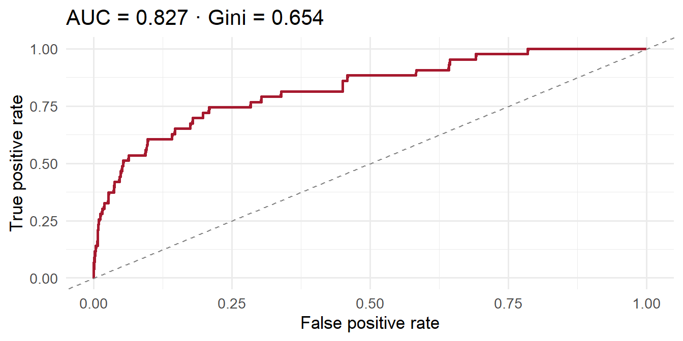
- AUC = probability that a randomly chosen defaulter is ranked above a randomly chosen non-defaulter.
- Gini = \(2 \cdot AUC - 1\). Bounded in \([0, 1]\); random model → 0; perfect model → 1.
- An AUC of 0.70 is deployable; 0.80+ is strong; above 0.95, suspect leakage.
Widget 4: ROC threshold slider
NoteWhy this matters
AUC measures ranking. But to deploy a model, you pick a threshold. Different thresholds → different costs. A default missed costs X; a good loan denied costs Y. The threshold is a business call, not a statistical one.
Move the threshold up: fewer false positives (good customers you denied), but more missed defaulters. Move it down: catch more defaulters, but deny a lot of good applicants. This tension is the whole job of a credit officer.
Part 5: Calibration
PIT PD vs long-run PD
- Logistic output = point-in-time (PIT) PD. Reflects current conditions; cycles.
- Basel III requires long-run PDs, that is multi-year averages, for capital. Pro-cyclicality is bad for stability.
- Calibration = mapping continuous PIT PDs into discrete grades, each with a long-run PD attached.
The calibrated rating table
| Grade | Description | PIT PD range | Long-run PD |
|---|---|---|---|
| AAA | Prime | 0.00 – 0.05% | 0.00% |
| AA | Very strong | 0.05 – 0.10% | 0.07% |
| A | Strong | 0.10 – 0.25% | 0.20% |
| BBB | Satisfactory | 0.25 – 0.75% | 0.60% |
| BB | Weak | 0.75 – 2.00% | 1.50% |
| B | Very weak | 2.00 – 5.00% | 3.50% |
| CCC | Distressed | 5.00 – 15.0% | 10.0% |
| CC | Highly distressed | 15.0 – 25.0% | 25.0% |
| C | Near default | ≥ 25.0% | 30.0% |
APS 113 floor. Every grade’s long-run PD must be at least 0.05% for capital. The AAA row above has PD = 0.00%, so for capital purposes we would floor it to 0.05%.
Widget 5: Rating bin tuner
NoteYou’re the credit committee
Drag the cut-points. Watch the grade distribution shift. In practice, calibration is a policy decision: tighter cutoffs mean fewer borrowers in top grades, which affects both RWA and commercial targeting.
Notice: when you narrow the AAA band, those borrowers spill into AA, increasing the count of a higher-risk grade, hence the bank’s RWA even if nothing changed in the underlying book. Calibration is not neutral.
Part 6: Validation
Transition matrix: old vs new ratings
Cross-tabulate old vs new ratings
calib_rating_labels <- c("AAA", "AA", "A", "BBB", "BB", "B", "CCC", "CC", "C")
calib_pd_breaks <- c(0, 0.0005, 0.001, 0.002, 0.007, 0.02, 0.05, 0.15, 0.25, 1)

credit_data$rating_new <- cut(
  credit_data$pd_pit_new,
  breaks = calib_pd_breaks, labels = calib_rating_labels,
  include.lowest = TRUE, right = TRUE
)

transition_mat <- table("Old" = credit_data$rating, "New" = credit_data$rating_new)
transition_prop <- round(prop.table(transition_mat, margin = 1) * 100, 1)

transition_df <- as.data.frame.matrix(transition_prop) |>
  tibble::rownames_to_column(var = "Old \\ New")

transition_df |>
  tt() |>
  style_tt(j = 1, align = "l", bold = TRUE) |>
style_tt(j = 2:10, align = "r")| Old \ New | AAA | AA | A | BBB | BB | B | CCC | CC | C |
|---|---|---|---|---|---|---|---|---|---|
| AAA | 3.0 | 1.0 | 8.0 | 50.0 | 37.0 | 1.0 | 0.0 | 0.0 | 0.0 |
| AA | 3.8 | 5.0 | 4.5 | 28.7 | 47.8 | 9.8 | 0.5 | 0.0 | 0.0 |
| A | 0.7 | 1.5 | 6.3 | 28.4 | 50.0 | 12.3 | 0.8 | 0.0 | 0.0 |
| BBB | 0.3 | 1.2 | 5.0 | 25.3 | 49.0 | 17.5 | 1.7 | 0.0 | 0.0 |
| BB | 0.0 | 0.1 | 1.5 | 17.9 | 45.4 | 28.5 | 6.5 | 0.0 | 0.0 |
| B | 0.1 | 0.0 | 0.1 | 5.3 | 31.1 | 37.7 | 22.7 | 2.5 | 0.5 |
| CCC | 0.0 | 0.0 | 0.0 | 1.2 | 14.7 | 28.8 | 39.3 | 11.7 | 4.3 |
| CC | 0.0 | 0.0 | 0.0 | 0.4 | 3.2 | 16.8 | 33.6 | 26.4 | 19.6 |
| C | 0.0 | 0.0 | 0.0 | 0.0 | 2.7 | 6.7 | 24.0 | 22.7 | 44.0 |
- Diagonal cells = borrowers whose grade is unchanged.
- A good model moves mass toward the diagonal. Wild dispersion = instability = recalibrate.
Widget 6: Transition matrix heatmap
RWA impact: does the new model hold up?
Apply irb_rwa() to each active loan under old and new ratings
irb_rwa <- function(PD, LGD, EAD, M, AVCM = 1) {
  PD <- pmax(PD, 0.0005)
  x <- (1 - exp(-50 * PD)) / (1 - exp(-50))
  R <- AVCM * (0.12 * x + 0.24 * (1 - x))
  b <- (0.11852 - 0.05478 * log(PD))^2
  term <- (qnorm(PD) + sqrt(R) * qnorm(0.999)) / sqrt(1 - R)
  K <- (LGD * pnorm(term) - PD * LGD) * ((1 + (M - 2.5) * b) / (1 - 1.5 * b))
  pmax(K, 0) * 12.5 * EAD
}

long_run_pd_table <- data.frame(
  rating      = calib_rating_labels,
  long_run_pd = c(0.0005, 0.0007, 0.0020, 0.0060, 0.0150, 0.0350, 0.10, 0.25, 0.30)
)

credit_data$pd_old <- long_run_pd_table$long_run_pd[match(credit_data$rating, long_run_pd_table$rating)]
credit_data$pd_new <- long_run_pd_table$long_run_pd[match(credit_data$rating_new, long_run_pd_table$rating)]

credit_data$maturity_year <- credit_data$year_borrowed + ceiling(credit_data$term_months / 12) - 1
active_loans <- credit_data |> filter(maturity_year >= current_year)

LGD <- 0.20
EAD <- active_loans$amount_in_thousands * 1000
M <- active_loans$term_months / 12

active_loans$rwa_old <- irb_rwa(active_loans$pd_old, LGD, EAD, M, 1)
active_loans$rwa_new <- irb_rwa(active_loans$pd_new, LGD, EAD, M, 1)

total_rwa_old <- sum(active_loans$rwa_old, na.rm = TRUE)
total_rwa_new <- sum(active_loans$rwa_new, na.rm = TRUE)
total_ead <- sum(EAD, na.rm = TRUE)
pct_change <- (total_rwa_new - total_rwa_old) / total_rwa_old * 100

tibble(
  Scenario       = c("Old ratings", "New ratings"),
  `Total EAD`    = c(total_ead, total_ead),
  `Total RWA`    = c(total_rwa_old, total_rwa_new)
) |>
  mutate(
    `Total EAD` = format(round(`Total EAD`), big.mark = ",", scientific = FALSE, trim = TRUE),
    `Total RWA` = format(round(`Total RWA`), big.mark = ",", scientific = FALSE, trim = TRUE)
  ) |>
  tt() |>
  style_tt(j = 1, align = "l") |>
style_tt(j = 2:3, align = "r")| Scenario | Total EAD | Total RWA |
|---|---|---|
| Old ratings | 138,559,930 | 73,144,324 |
| New ratings | 138,559,930 | 84,600,942 |
The new model shifts total RWA by +15.66%. A bank signs off or sends the model back for recalibration based on this number and the stability of ratings.
Part 7: Classic scoring models (bonus)
Before logit: Altman’s Z-score (1968)
Ed Altman fit a discriminant function on US manufacturers:
\[ Z = 1.2 X_1 + 1.4 X_2 + 3.3 X_3 + 0.6 X_4 + 1.0 X_5 \]
where
- \(X_1=\) Working capital / Total assets
- \(X_2=\) Retained earnings / Total assets
- \(X_3=\) EBIT / Total assets
- \(X_4=\) Market equity / Book liabilities
- \(X_5=\) Sales / Total assets
Zones:
- \(Z < 1.81\) → distressed
- \(1.81 \le Z < 2.99\) → grey
- \(Z \ge 2.99\) → safe
Widget 7: Altman Z-score calculator
Z-score is an accounting-data scorecard, with no market prices required. That’s its appeal for private firms. Its weakness is that the coefficients were fit on a small sample of US manufacturers with bankruptcies filed between 1946 and 1965; they are not universal across countries, industries or eras.
Merton’s structural model (1974)
Treat the firm as a call option on its assets:
- Assets \(V\) evolve as geometric Brownian motion with volatility \(\sigma\).
- Debt \(D\) matures at horizon \(T\).
- Equity \(=\) \(\max(V_T - D, 0)\), a call option on assets.
- Default at \(T\) if \(V_T < D\).
\[ d_2 = \frac{\ln(V/D) + (r - \sigma^2/2)\,T}{\sigma\sqrt{T}}, \qquad PD = N(-d_2) \]
Widget 8: Merton distance-to-default
Two worldviews for the same number. Logit says “PD is a function of accounting ratios.” Merton says “PD is implied by the firm’s market-value capital structure.” Moody’s KMV commercialised Merton; Basel IRB expects logit-style empirical models. Real banks often blend both.
Part 8: Knowledge check
Quiz 1
If PD doubles from 1.0% to 2.0%, does RWA double?
No. The risk-weight function is non-linear in PD, via correlation \(R\), the maturity adjustment \(b\), and the normal-CDF term. Use Widget 1 to check: at the default settings, RWA approximately increases by ~50% when PD doubles from 1% → 2%, not 100%.
Quiz 2
Our fitted model above scored AUC ≈ 0.83 (Gini ≈ 0.65) on held-out data. A colleague says “great, we’re ready to deploy.” Are they?
Not by itself. AUC ≈ 0.83 is a respectable discrimination number, but discrimination is only one of four pillars. Before deployment you also need:
- Calibration: do predicted PDs match the realised default rates per grade? A well-ranked model can still be systematically off.
- Threshold economics: Widget 4 shows the false-positive / false-negative trade-off. The right threshold depends on the cost of missed defaulters vs denied good loans.
- Stability: Widget 6 and the transition matrix: does the new model re-grade borrowers sensibly, or does it churn them across grades?
- RWA impact: will the new model’s long-run PDs blow through the capital budget?
A headline AUC number is a necessary condition, not a sufficient one.
Quiz 3
In our transition matrix (Table 8), only ~3% of old-AAA borrowers remain AAA under the new model, and about 50% are re-graded all the way down to BBB. About 49% of old-BBB loans drop to BB. Good news or bad?
Red flag either way, and it needs a story. A three-notch downgrade concentrated at the prime end of the book is exactly the kind of shift a regulator will ask about:
- If the old AAAs really were prime, the new model is broken at the high end, so investigate the coefficients driving low-PD scores.
- If the old AAAs were never really AAA, the old model was too generous and the bank was under-capitalised. This is a correction, but one that must come with a provisioning and capital-planning story.
The large one-notch drift across the whole book (old-BBB → new-BB, old-A → new-BB) says the new model is systematically more conservative. You don’t deploy a model with this much migration without (a) understanding which story applies and (b) stress-testing the RWA impact (Table 9).
Quiz 4
Why does IRB capital \(K\) fall when PD goes above ~30%?
Because K covers unexpected loss, not expected loss. When default is almost certain, the loss is expected, so it belongs in provisioning (IFRS 9) rather than capital. The “surprise” component, which is what capital funds, shrinks as PD approaches 1.
Wrap-up
Key takeaways
- RWA = K × 12.5 × EAD is the business end of credit-risk modelling. Everything before it, from simulating to screening, fitting, calibrating and validating, feeds one number.
- PIT vs long-run PD. Logit outputs are PIT; Basel capital needs long-run. Calibration is the bridge, and it’s a policy choice.
- Model quality is three things, not one. Discrimination (AUC) + calibration + stability. Skip any one and you will be told about it.
- Capital ≠ provisioning. Expected loss lives in provisions (IFRS 9). Unexpected loss lives in capital (Basel). Don’t double-count.
- Structural vs empirical. Merton and logit answer the same question from different directions. Use both when you can.
Resources
- Full narrative version: Credit Risk Modelling (IRB)
- APRA Prudential Standard APS 113: Capital Adequacy, IRB Approach to Credit Risk
- BIS Basel framework CRE32: IRB approach and risk components
- Altman, E. I. (1968). “Financial Ratios, Discriminant Analysis and the Prediction of Corporate Bankruptcy.” Journal of Finance.
- Merton (1974) (structural approach)
- Gorton and He (2008)
References
Gorton, G B, and Ping He. 2008. “Bank Credit Cycles.” Review of Economic Studies 75 (4): 1181–214.
Merton, Robert C. 1974. “On the Pricing of Corporate Debt: The Risk Structure of Interest Rates*.” The Journal of Finance 29 (2): 449–70. https://doi.org/10.1111/j.1540-6261.1974.tb03058.x.
Footnotes
This means that the computed RWAs may receive additional scaling or other adjustments as specified by the APS 113.↩︎