Probability of Informed Trading (PIN)

Note

This post was originally published on my old blog in March 2018 in Chinese. Translation is provided by ChatGPT-4.

The above figure is based on data I collected in 2019 of trades on Binance.

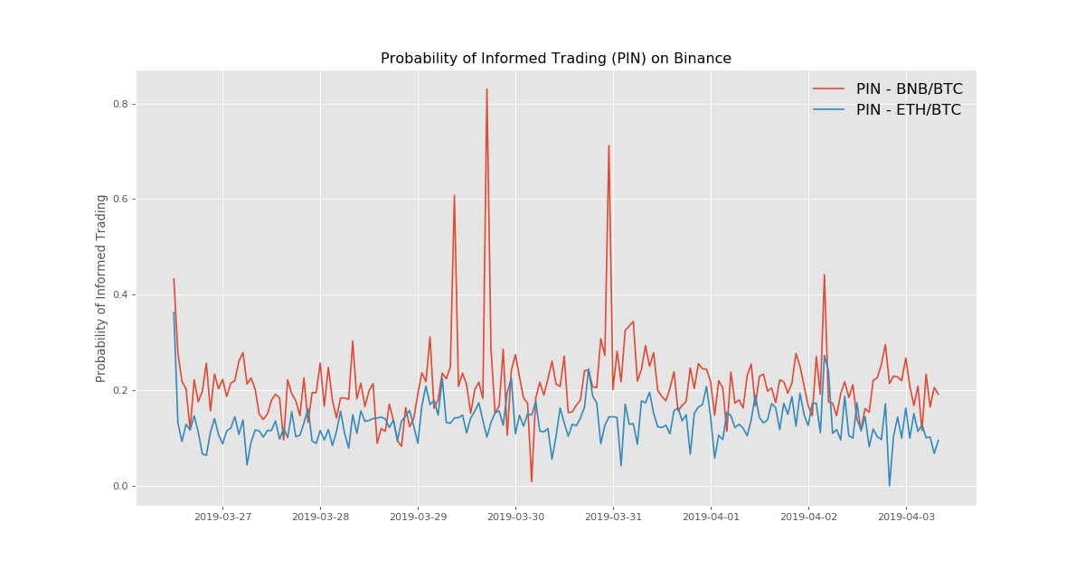
In the market microstructure literature, Easley et. al. (1996) proposed a trading model that can decompose the bid-ask spread. The most commendable aspect of this model is the introduction of the "Probability of Informed Trading," or PIN, which serves as a means of measuring the informational component in the spread. As the name suggests, under ideal conditions, PIN can reflect the probability of informed trading in a market with market maker. In this article, I attempt to comb through the modeling process in the Easley et. al. (1996) paper and discuss how to handle the objective function in maximum likelihood estimation to avoid overflow errors during computation.

Model

Assume that the buy and sell orders of informed and uninformed traders follow independent Poisson processes, and the following tree diagram describes the entire trading process:

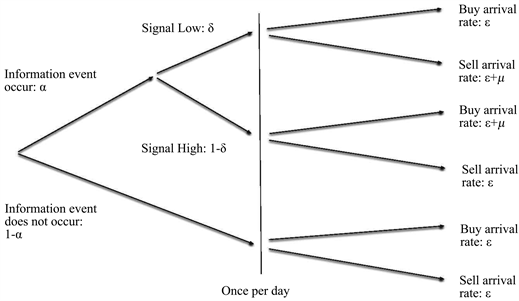
• On each trading day, there is a probability of \(P=\alpha\) that new information will appear, and obviously a probability of \(P=(1-\alpha)\) that there will be no new information.
• The probability of new information being bearish is \(P=\delta\), and the probability of it being bullish is \(P=(1-\delta)\).
• If the news is bearish, the arrival rate of buy orders on that day is \(\varepsilon\), and the arrival rate of sell orders is \((\varepsilon+\mu)\).
• If the news is bullish, the arrival rate of buy orders on that day is \((\varepsilon+\mu)\), and the arrival rate of sell orders is \(\varepsilon\).
• When there is no new information, the arrival rate of both buy and sell orders is \(\varepsilon\).

Trading Process

Next, assume that the market maker is a Bayesian, that is, he will update his understanding of the overall market status, especially whether there is new information on that day, by observing trades and trading rates. Suppose each trading day is independent, \(P(t)=(P_n(t), P_b(t), P_g(t))\) is the market maker's prior probability perception, where \(n\) represents no new information, \(b\) represents bearish bad news, and \(g\) represents bullish good news, so \(P(t)=(1-\alpha, \alpha\delta, \alpha(1-\delta))\).

Let \(S_t\) be the event of a sell order arriving at time \(t\), and \(B_t\) be the event of a buy order arriving at time \(t\). Also, let \(P(t|S_t)\) be the updated probability perception of the market maker after observing a sell order arriving at time \(t\) based on the existing information. Then, according to Bayes' theorem, if there is no new information at time \(t\) and the market maker observes a sell order, the posterior probability \(P_n(t|S_t)\) should be:

\[ \begin{equation} P_n(t|S_t)=\frac{P_n(t)\varepsilon}{\varepsilon+P_b(t)\mu}\end{equation} \]

Similarly, if there is bearish information and the market maker observes a sell order at time \(t\), the posterior probability \(P_b(t|S_t)\) should be:

\[ \begin{equation} P_b(t|S_t)=\frac{P_b(t)(\varepsilon+\mu)}{\varepsilon+P_b(t)\mu}\end{equation} \]

If there is bullish information and the market maker observes a sell order at time \(t\), the posterior probability \(P_g(t|S_t)\) should be:

\[ \begin{equation} P_g(t|S_t)=\frac{P_g(t)\varepsilon}{\varepsilon+P_b(t)\mu} \end{equation} \]

Thus, the expected zero-profit bid price at time \(t\) on day \(i\) should be the conditional expectation of the asset value based on historical information and observing sell order at this time, that is,

\[ \begin{equation} b(t)=\frac{P_n(t)\varepsilon V^*_i+P_b(t)(\varepsilon+\mu)\underline{V}_i+P_g(t)\varepsilon\overline{V}_i}{\varepsilon+P_b(t)\mu} \end{equation} \]

Here, \(V_i\) is the value of the asset at the end of day \(i\), and let the asset value be \(\overline{V}_i\) when there is positive news, \(\underline{V}_i\) when there is negative news, and \(V^*_i\) when there is no news, with \(\underline{V}_i < V^*_i < \overline{V}_i\).

At this point, the ask price should be:

\[ \begin{equation} a(t)=\frac{P_n(t)\varepsilon V^*_i+P_b(t)\varepsilon\underline{V}_i+P_g(t)(\varepsilon+\mu)\overline{V}_i}{\varepsilon+P_g(t)\mu}\end{equation} \]

Let's associate these bid and ask prices with the expected asset value at time \(t\). Considering that the conditional expectation of the asset value at this time is:

\[ \begin{equation} E[V_i|t]=P_n(t)V^*_i+P_b(t)\underline{V}_i+P_g(t)\overline{V}_i\end{equation} \]

we can write the above \(b(t)\) and \(a(t)\) as:

\[ \begin{equation} b(t)=E[V_i|t]-\frac{\mu P_b(t)}{\varepsilon+\mu P_b(t)}(E[V_i|t]-\underline{V}_i)\end{equation} \]

\[ \begin{equation} a(t)=E[V_i|t]+\frac{\mu P_g(t)}{\varepsilon+\mu P_g(t)}(\overline{V}_i-E[V_i|t])\end{equation} \]

Thus, the bid-ask spread is \(a(t)-b(t)\), which is:

\[ \begin{equation} a(t)-b(t)=\frac{\mu P_g(t)}{\varepsilon+\mu P_g(t)}(\overline{V}_i-E[V_i|t])+\frac{\mu P_b(t)}{\varepsilon+\mu P_b(t)}(E[V_i|t]-\underline{V}_i)\end{equation} \]

This indicates that the bid-ask spread at time \(t\) is actually:

The probability of a buy order being an informed trade \(\times\) the expected loss due to the informed buyer + the probability of a sell order being an informed trade \(\times\) the expected loss due to the informed seller

Therefore, the probability that any trade at time \(t\) is based on asymmetric information from informed traders is the sum of these two probabilities:

\[ \begin{equation} PIN(t)=\frac{\mu P_g(t)}{\varepsilon+\mu P_g(t)}+\frac{\mu P_b(t)}{\varepsilon+\mu P_b(t)}=\frac{\mu(1-P_n(t))}{\mu(1-P_n(t))+2\varepsilon}\end{equation} \]

If no information event occurs (\(P_n(t)=1\)) or there are no informed trades (\(\mu=0\)), both \(PIN\) and the bid-ask spread should be zero. If the probabilities of positive and negative news are equal, i.e., \(\delta=1-\delta\), the bid-ask spread can be simplified to:

\[ \begin{equation} a(t)-b(t)=\frac{\alpha\mu}{\alpha\mu+2\varepsilon}[\overline{V}_i-\underline{V}_i]\end{equation} \]

And our \(PIN\) measure is simplified to:

\[ \begin{equation} PIN(t)=\frac{\alpha\mu}{\alpha\mu+2\varepsilon}\end{equation} \]

Model Estimation

After the model is established, let's talk about the parameter estimation of this model. The parameters we need to estimate, \(\theta=(\alpha, \delta, \varepsilon, \mu)\), are actually very difficult to estimate. This is because we cannot directly observe them, and can only observe the arrival of buy and sell orders. In this model, the daily buy and sell orders are assumed to follow one of the three Poisson processes. Although we don't know which process it is specifically, the overall idea is: more buy orders imply potential good news, more sell orders imply potential bad news, and overall buying and selling will decrease when there is no new information. With this idea in mind, we can try to estimate \(\theta\) using the maximum likelihood estimation method.

First, according to the trading model shown in the diagram, assume that there is bad news on a certain day, then the arrival rate of sell orders is \((\mu+\varepsilon)\), which means both informed and uninformed traders participate in selling. The arrival rate of buy orders is \(\varepsilon\), that is, only uninformed traders will continue to buy. Therefore, the probability of observing a sequence of trades with \(B\) buy orders and \(S\) sell orders in a period of time is:

\[ \begin{equation} e^{-\varepsilon} \frac{\varepsilon^B}{B!} e^{-(\mu+\varepsilon)} \frac{(\mu+\varepsilon)^S}{S!} \end{equation} \]

If there is good news on a certain day, the probability of observing a sequence of trades with \(B\) buy orders and \(S\) sell orders in a period of time is:

\[ \begin{equation} e^{-\varepsilon} \frac{\varepsilon^B}{B!} e^{-\varepsilon} \frac{\varepsilon^S}{S!} \end{equation} \]

If there is no new information on a certain day, the probability of observing a sequence of trades with \(B\) buy orders and \(S\) sell orders in a period of time is:

\[ \begin{equation} e^{-(\mu+\varepsilon)} \frac{(\mu+\varepsilon)^B}{B!} e^{-\varepsilon} \frac{\varepsilon^S}{S!} \end{equation} \]

So, the probability of observing a total of \(B\) buy orders and \(S\) sell orders on a trading day should be the weighted average of the above three possibilities, and the weights here are the probabilities of each possibility. Therefore, we can write out the likelihood function:

\[ \begin{align} L((B, S)| \theta)=  &(1-\alpha)e^{-\varepsilon} \frac{\varepsilon^B}{B!} e^{-\varepsilon} \frac{\varepsilon^S}{S!} \\ &+ \alpha\delta  e^{-\varepsilon} \frac{\varepsilon^B}{B!} e^{-(\mu+\varepsilon)} \frac{(\mu+\varepsilon)^S}{S!} \\ &+ \alpha(1-\delta) e^{-(\mu+\varepsilon)} \frac{(\mu+\varepsilon)^B}{B!} e^{-\varepsilon} \frac{\varepsilon^S}{S!} \end{align} \]

Hence, the objective function of the maximum likelihood function is:

\[ \begin{equation} L(D|\theta)=\prod_{i=1}^{N}L(\theta|(B_i, S_i)) \end{equation} \]

Bottomline

The problem seems to end here. With the objective function, it seems to be all set as long as you program it and pay attention to the parameter boundaries. However, the real challenge comes next, because if you really write the objective function like this and run it, you will inevitably encounter an overflow error. After all, this function is filled with powers and factorials. Even if the time element is chosen very small, some highly liquid assets will still have hundreds of transactions within a few seconds. Therefore, both \(B!\), \(S!\), and \((\mu+\varepsilon)^B\) can beautifully crash your program. So, further processing of the objective function here is extremely important.

By observing equation (16), the three terms in the likelihood function can actually extract a common factor \(e^{-2\varepsilon}(\mu+\varepsilon)^{B+S}/(B!S!)\)! After extracting this common factor, you can also substitute \(x\equiv \frac{\varepsilon}{\mu+\varepsilon}\in [0, 1]\) into it. The transformed likelihood function, after taking the logarithm, will be in the form:

\[ \begin{align} l((B, S)| \theta)=&\ln(L((B, S)| \theta))\\ =&-2\varepsilon+(B+S)\ln(\mu+\varepsilon) \\ &+\ln((1-\alpha)x^{B+S}+\alpha\delta e^{-\mu}x^B + \alpha(1-\delta)e^{-\mu}x^S) \\ &-\ln(B!S!) \end{align} \]

Now, since the last term \(\ln(B!S!)\) does not affect the parameter estimation at all, it can be safely excluded. The remaining part can perfectly avoid overflow. Personally, I think the brilliant move here is the introduction of \(x\equiv \frac{\varepsilon}{\mu+\varepsilon}\in [0, 1]\), which prevents the overflow error caused by \((\mu+\varepsilon)>1\).

Comments