FRED - Federal Reserve Economic Data
Since Stata 15, we can search, browse and import almost a million U.S. and international economic and financial time series made available by the St. Louis Federal Reserve's Federal Research Economic Data. This post briefly explains this great feature.
Prerequisite
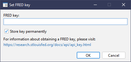
Before you start, you will need an API Key from FRED. Register one here
Then in Stata, you can store this key permanently so you don't need to provide again.(1)
- Replace
_key_with your actual API Key obtained.
GUI is always a good start
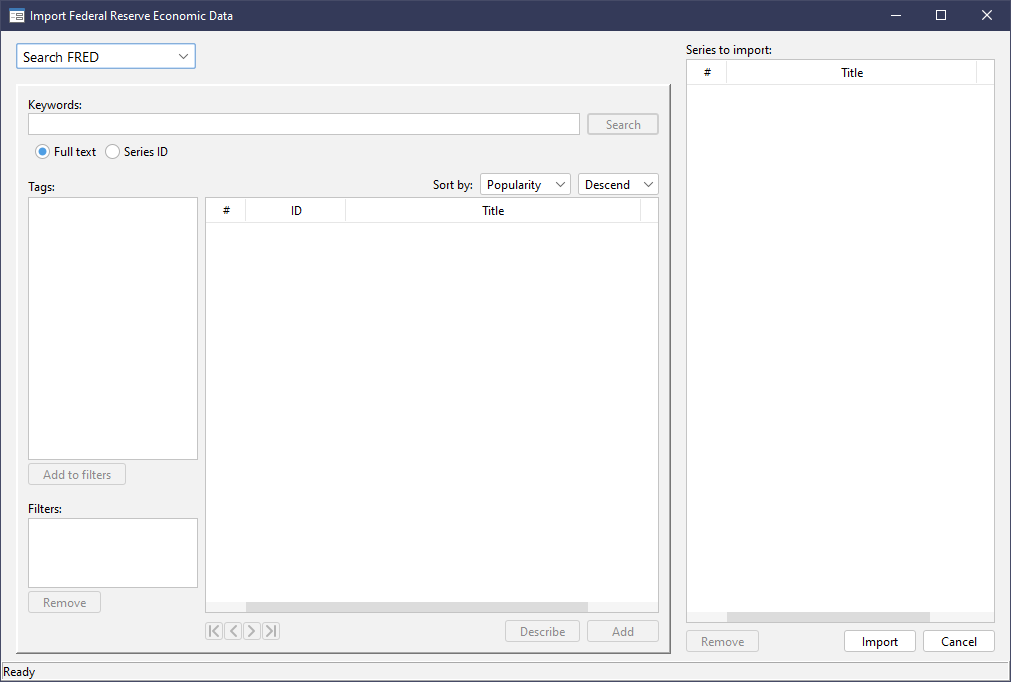
Alternatively, click on menu File>Import>Fedearl Reserve Economic Data (FRED) will bring up the dialog as shown below.
Enter API Key and you'll be free to explore all the data series available on FRED.
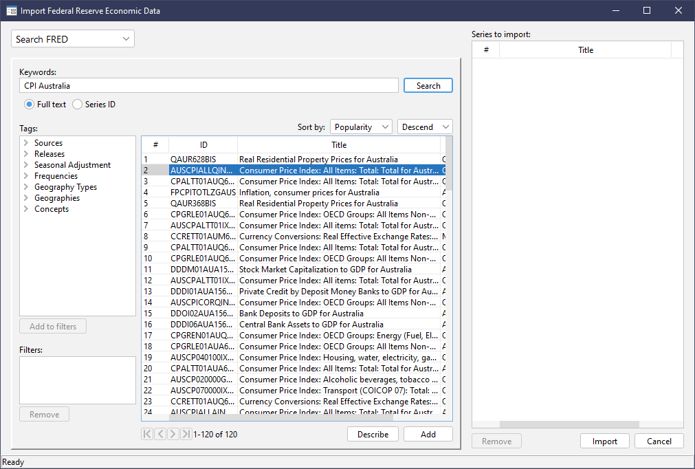
For example, let's see the CPI of Australia...
Describe the data series, we can find many useful meta info.
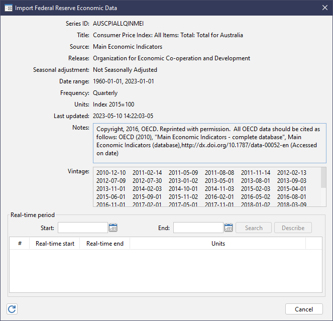
Vintage
Note that "vintage" section lists a number of dates, with each vintage referring a particular version of the data series at that point of time.
It may sound strange but an economic data series may be revised multiple times after it has been published. Potential reasons may be that later people collect more accurate information, or that there is a change of estimation method, etc.
For example, the CPI from 2005 to 2010 collected by a research as at 2011 may be different from the one collected as at 2023. Without specifying the data vintage, replicating a prior work can be hard.
Another tricky part is that ignoring vintages introduces look-ahead bias in analysis.
For example, a trading strategy using the revised GDP accessed today, instead of the vintage GDP, implicitly uses hindsight as the GDP series may have been revised to accomodate more accurate data obtained after release.
Let's close the description, double click on the series and click on import. Another dialog will be shown to confirm some final details.
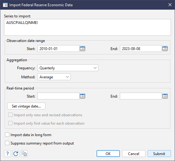
The outputs will be like the following:
. import fred AUSCPIALLQINMEI, daterange(2010-01-01 2023-08-08) aggregate(quarterly,avg)

Summary
----------------------------------------------------------------------------------------------------------------------------------------------------------------------------------------------------------------
Series ID                    Nobs    Date range                Frequency
----------------------------------------------------------------------------------------------------------------------------------------------------------------------------------------------------------------
AUSCPIALLQINMEI              53      2010-01-01 to 2023-01-01  Quarterly
----------------------------------------------------------------------------------------------------------------------------------------------------------------------------------------------------------------
# of series imported: 1
   highest frequency: Quarterly
    lowest frequency: Quarterly
Programmatical is recipe to reproducibility
We don't need to go through the GUI process every time. In fact, Stata already told us what the corresponding command is:
We can simply put this line of code into our program.
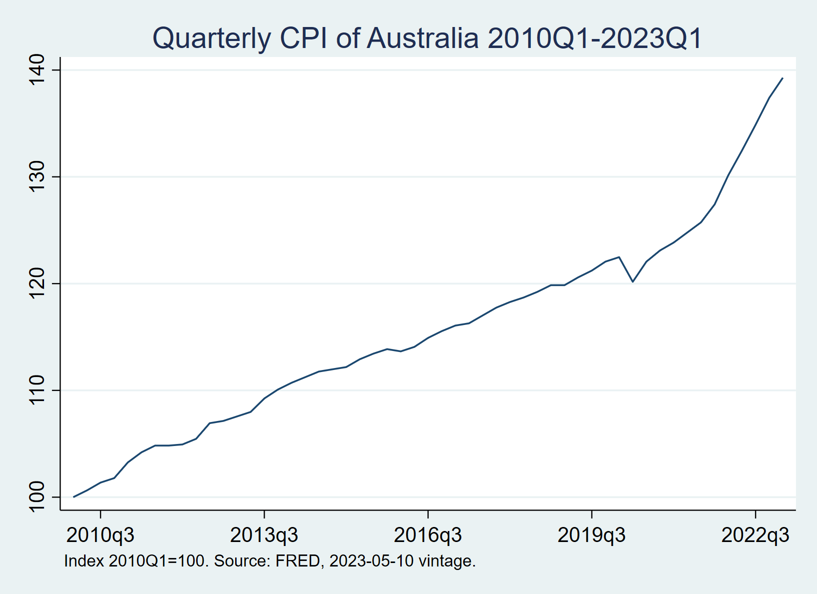
For example, the code below generates a time-series chart for Australia's CPI.
// Import
import fred AUSCPIALLQINMEI, daterange(2010-01-01 2023-03-31) vintage(2023-05-10) aggregate(quarterly,avg) clear
rename AUSCPIALLQINMEI_20230510 cpi_australia
// Time format
gen yrqtr = yq(year(daten),quarter(daten))
format yrqtr %tq
tsset yrqtr
// Set start of the period to 100
gen cpi_ret = cpi_australia/L.cpi_australia - 1
replace cpi_australia = 100 if _n==1
replace cpi_australia = L.cpi_australia * (1+cpi_ret) if _n>1
// Plotting
twoway (tsline cpi_australia), title("Quarterly CPI of Australia 2010Q1-2023Q1") ytitle("") ttitle("") note("Index 2010Q1=100. Source: FRED, 2023-05-10 vintage.")
Note
The code snippet above specifies the data vintage. Therefore, even if someone runs it 30 years from now, they will still get exactly the same data and plot as I do in 2023.