Difference-in-Differences Estimation
Empirical researchers have been using difference-in-differences (DiD) estimation to identify an event's Average Treatment effect on the Treated entities (ATT). This post is my understanding and a non-technical note of the DiD approach as it evolves over the past years, especially on the problems and solutions when multiple treatment events are staggered.
One event and the canonical DiD
The canonical DiD takes a \(2\times 2\) form which involves 2 periods (before & after) and 2 groups (treated and untreated). Under the assumption of parallel trends (1), the most common approach to identify ATT is a two-way fixed effect (TWFE) linear regression.
- Parallel trends assume that the change in the outcomes of treated group, in absence of the treatment, is the same as the change in the outcomes of the untreated group.
Specifically, we would estimate the following model:
where \(Y_{it}\) is the outcome of interest for entity \(i\) at time \(t\), \(D_{it}\) is an indicator that takes the value of 1 if entity \(i\) has been treated at time \(t\)(1), \(\theta_t\) is the time fixed effect and \(\gamma_i\) is the entity fixed effect (2). Here, estimate of \(\beta\) is interpreted as the ATT.
- If we have separate \(\text{Treatment}_i\) and \(\text{Post}_{t}\) indicators, then \(D_{it}=\text{Treatment}_i \times \text{Post}_t\).
- The presence of time and entity fixed effects absorbs individual \(\text{Post}_t\) and \(\text{Treatment}_{i}\) variables in the model.
This TWFE method works when
- There is homogeneous treatment effect, i.e., the treatment effect is the same for all treated entities.
- There is only one treatment event such that we have only two periods (before and after the treatment). In this case, TWFE is robust to treatment effect heterogeneity. That is, even though the treatment effect may not be the same for all treated entities, the estimated \(\beta\) is numerically equal to the ATT.
What if there are multiple treatments at different times?
Problems of TWFE with multiple events
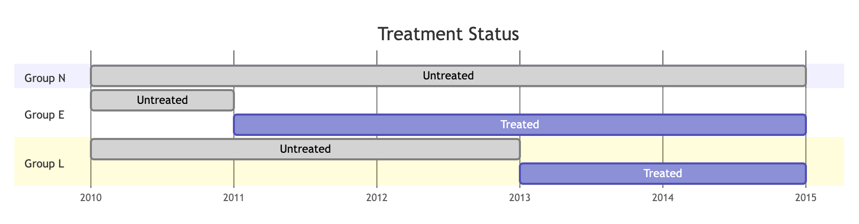
Suppose there are two treatment events. Let's visualize the treatment status of three groups of entities, the Never-treated group N, the Early-treated group E and the Late-treated group L. Here I ignore the possibility that a group has always been treated.
Goodman-Bacon (2021) shows that, in this case, TWFE estimate of \(\beta\) in Equation (1) above is in fact a (complicated) weighted-average of all possible \(2\times2\) DiD estimates, which leads to bias:
- For the event to group E (Early-treated):
- E vs N. No problem, controls are never treated.
- E vs L. No problem, controls have not yet been treated.
- For the event to group L (Late-treated):
- L vs N. No problem, controls are never treated.
- L vs E. Problematic, controls have been treated (by another earlier event).(1)
- This may not seem obvious given that group E would have \(D_{it}=1\) after 2011. But DiD is actually comparing the "before-after" differences in outcomes of entities whose treatment statuses just change to those whose treatment statuses do not change. The already-treated group E's status stay unchanged from 2011 to 2014.
What to do then? An overview
When there is a staggered adoption design, i.e., groups of entities receive treatments in a staggered way, there are a few modified DiD approaches that try to produce ATT estimates robust to the bias. But the key idea is to avoid including as controls the entities that have been previously treated, then find a good way to aggregate the many estimates as a result of multiple events. Here I discuss two approaches, namely stacked DiD and CS DiD.
Stacked DiD tries to solves the issue by essentially "selecting only good controls". Specifically, for each treatment event, we construct a cohort of treated and untreated entities, where the "untreated" are those never treated and/or those not yet treated by any prior treatment. Cohorts are then stacked together in regression. To my knowledge, Gormley and Matsa (2011) and Gormley, Matsa and Milbourn (2013) already use a stacked DiD. Some later papers using stacked DiD include, for example, Cengiz, Dube, Lindner and Zipperer (2019), Deshpande and Li (2019), among many others.
CS DiD (Callaway and Sant'Anna (2021)) groups entities by their treatment time and estimates each group's ATT at each time period since its treatment to the end of the sample period, also using never treated entities or those not yet treated. The many group-time ATTs are then aggregated to various levels for understanding the treatment effect. As at August 2023, CS DiD has already been cited over 3,000 times based on Google Scholar.
Stacked DiD
Centre to stacked DiD is the idea of building cohorts of clean \(2\times2\) DiD pairs, within each the entities used as controls are guaranteed to be not treated previously.
For a stacked DiD, we estimate a regression specification like below:
where
- \(Treat_{ic}\) is an indicator that equals 1 if entity \(i\) in cohort \(c\) is treated.
- \(Post_{ct}\) is an indicator that equals 1 if time period \(t\) in cohort \(c\) is after treatment event.
Alternatively and preferably (?), replace \(Treat_{ci}\) and \(Post_{ct}\) with cohort-entity fixed effect \(\gamma_{ic}\) and cohort-time fixed effect \(\theta_{ct}\):
where \(D_{ict}\equiv Treat_{ic}\times Post_{ct}\) is an indicator that equals 1 if entity \(i\) in cohort \(c\) has been treated at time \(t\).
Comparison with one-period TWFE
Easy to notice that Equation (3) is very similar to Equation (1). Instead of using an entity-time level indicator \(D_{it}\) in TWFE Equation (1) to estimate ATT, stacked DiD uses an entity-cohort-time level indicator \(D_{ict}\). Time and entity fixed effects are also allowed to vary across cohorts.
Stacked DiD effectively pool together ATT estimates from only good \(2\times2\) DiD pairs, thereby avoiding the bias caused by simple TWFE when treatment events are staggered.
Stacked DiD by construction causes duplication of observations since an entity-time can be used as control in different cohorts, which means observations in the stacked dataset can be correlated. We need to use proper clustering to address it, usually done by clustering at the entity level.
An event-study form of stacked DiD can further help identifying the time-varying treatment effects. Specifically, we replace the cohort-time \(Post_{ct}\) indicator with a series of cohort-time dummy variables, e.g., \(\{..., d^{-2}_{ct}, d^{-1}_{ct}, d^{0}_{ct}, d^{1}_{ct}, d^{2}_{ct}, ... \}\), where \(d^{\tau}_{ct}=1\) if time \(t\) in cohort \(c\) is \(\tau\) periods after (or before, if negative) the treatment. So, we will have
The estimates \(\{\beta_{\tau}\}\) can describe the time-varying treatment effect, i.e., the difference between treated and control in outcome \(Y\), \(\tau\) periods after the treatment.
Callaway and Sant'Anna (CS) DiD
Callaway and Sant'Anna (2021) (CS) DiD groups entities by their treatment time and estimates each group's ATT at each time since treatment to the end of the sample period, similarly using never treated (or not yet treated) as control.
How it works?
Intuitively, ATT (Average Treatment effect on the Treated) is an expected difference between the outcome if treated \(Y(1)\) and the outcome if untreated \(Y(0)\), for the treated entities (\(D=1\)).
CS DiD builds a group-time ATT, the expected difference in the outcome if treated in group \(g\) \(Y(g)\) and the outcome if untreated \(Y(0)\), for the treated entities in group \(g\) (\(G=g\)).
This is the average effect of participating in the treatment for entities in group \(g\) at time period \(t\).
Example
In the example above, we will have many group-time ATTs:
- 2011 group: \(ATT^{g=2011}_{t=2010}\), \(\color{blue}ATT^{g=2011}_{t=2011}\), \(\color{blue}ATT^{g=2011}_{t=2012}\), \(\color{blue}ATT^{g=2011}_{t=2013}\), \(\color{blue}ATT^{g=2011}_{t=2014}\), and \(\color{blue}ATT^{g=2011}_{t=2015}\).
- 2013 group: \(ATT^{g=2013}_{t=2010}\), \(ATT^{g=2013}_{t=2011}\), \(ATT^{g=2013}_{t=2012}\), \(\color{blue}ATT^{g=2013}_{t=2013}\), \(\color{blue}ATT^{g=2013}_{t=2015}\), and \(\color{blue}ATT^{g=2013}_{t=2015}\).
The blue-coloured ATTs are of interest to us to study the treatment effect. We can aggregate these ATTs by group \(g\), by calendar time \(t\), by relative time to events, or to a single overal measure of the treatment effect.
With the many group-time ATT estimates, CS DiD then proposes several aggregation ways to highlight treatment effect heterogeneity or to overall treatment effect parameters, enabling studies on:
- How do average treatment effects vary with length of exposure to the treatment?
- How do average treatment effects vary across groups?
- What is the cumulative average treatment effect of the policy across all groups until some time \(\tilde{t}\)?
- What is a general-purpose summary of the ATT?
A bit more details
To me, CS DiD and stacked DiD share some similarities.
Stacked DiD select "good controls" into groups. While it will create many duplicates, we may use propensity score matching (PSM) to mitigate the problem, which also helps with the parallel trend assumption (conditional on covariates).
CS DiD does not select "good controls" into groups. Instead, CS DiD estimates group-time ATTs by aggregating the "before-after" differences of entities base on entities' treatment status and their propensity to be treated in the group, etc. For example, the inverse-probability-weighting estimand for \(ATT(g,t)\) is given by
where \(P_g\equiv\frac{p_g(X)C}{1-p_g(X)C}\) is like a propensity score ratio; \(p_g(X)\) is the propensity score of an entity being treated at the time defined by group \(g\), conditional on the pre-event covariates \(X\); \(C=1\) if an entity does not participate in the treatment and zero otherwise; \(G_g=1\) if an entity is in group \(g\) (i.e., treated at the time defined by group \(g\)) and zero otherwise.(1)
- In comparison, a TWFE DiD aggregates the "before-after" differences by giving a weight of +1 to treated entities and -1 to controls.
How do they compare?
Warning
This is NOT a comprehensive test in terms of their performance. The stacked DiD code is written in a few minutes and so may contain errors.
The Stata -csdid- command comes very handy. I'm to use its help file and demo dataset to do some quick showcases.
CS DiD
use https://friosavila.github.io/playingwithstata/drdid/mpdta.dta, clear

csdid lemp, ivar(countyreal) time(year) gvar(first_treat) method(dripw) wboot rseed(1) agg(simple)
The output is:
............
Difference-in-difference with Multiple Time Periods

                                                         Number of obs = 2,500
Outcome model  : least squares
Treatment model: inverse probability
---------------------------------------------------------------------
            | Coefficient  Std. err.      t      [95% conf. interval]
------------+--------------------------------------------------------
        ATT |  -.0399513   .0121272    -3.29    -.0647386    -.015164
---------------------------------------------------------------------
Control: Never Treated

See Callaway and Sant'Anna (2021) for details
Additional results
. estat all
Test will be based on asymptotic VCoV
If you want aggregations based on WB, use option saverif() ad csdid_stats
Pretrend Test. H0 All Pre-treatment are equal to 0
chi2(5) =     7.7912
p-value  =     0.1681
Average Treatment Effect on Treated
------------------------------------------------------------------------------
            | Coefficient  Std. err.      z    P>|z|     [95% conf. interval]
-------------+----------------------------------------------------------------
        ATT |  -.0399513    .012034    -3.32   0.001    -.0635375    -.016365
------------------------------------------------------------------------------
ATT by group
------------------------------------------------------------------------------
            | Coefficient  Std. err.      z    P>|z|     [95% conf. interval]
-------------+----------------------------------------------------------------
    GAverage |  -.0310183   .0123872    -2.50   0.012    -.0552967   -.0067399
    G2004 |  -.0797491   .0263678    -3.02   0.002    -.1314291   -.0280692
    G2006 |  -.0229095   .0167033    -1.37   0.170    -.0556475    .0098284
    G2007 |  -.0260544   .0166554    -1.56   0.118    -.0586985    .0065896
------------------------------------------------------------------------------
ATT by Calendar Period
------------------------------------------------------------------------------
            | Coefficient  Std. err.      z    P>|z|     [95% conf. interval]
-------------+----------------------------------------------------------------
    CAverage |  -.0417004   .0159719    -2.61   0.009    -.0730047   -.0103962
    T2004 |  -.0105032    .023251    -0.45   0.651    -.0560744    .0350679
    T2005 |  -.0704232   .0309848    -2.27   0.023    -.1311522   -.0096941
    T2006 |   -.048816   .0201259    -2.43   0.015    -.0882619     -.00937
    T2007 |  -.0370593   .0137471    -2.70   0.007    -.0640031   -.0101156
------------------------------------------------------------------------------
ATT by Periods Before and After treatment
Event Study:Dynamic effects
------------------------------------------------------------------------------
            | Coefficient  Std. err.      z    P>|z|     [95% conf. interval]
-------------+----------------------------------------------------------------
    Pre_avg |   .0018283    .007657     0.24   0.811    -.0131791    .0168357
    Post_avg |  -.0772398    .019965    -3.87   0.000    -.1163705   -.0381092
        Tm3 |   .0305067   .0150336     2.03   0.042     .0010414    .0599719
        Tm2 |  -.0005631   .0132916    -0.04   0.966    -.0266142    .0254881
        Tm1 |  -.0244587   .0142364    -1.72   0.086    -.0523616    .0034441
        Tp0 |  -.0199318   .0118264    -1.69   0.092    -.0431111    .0032474
        Tp1 |  -.0509574   .0168935    -3.02   0.003     -.084068   -.0178468
        Tp2 |  -.1372587   .0364357    -3.77   0.000    -.2086713   -.0658461
        Tp3 |  -.1008114   .0343592    -2.93   0.003    -.1681542   -.0334685
------------------------------------------------------------------------------
Stacked DiD
For stacked DiD, I use the following code.
frame copy default events, replace
frame change events

keep first_treat
keep if first_treat != 0
duplicates drop
sort first_treat
di "3 events in 2004, 2006, 2007 respectively"

cap frame drop did
mkf did

// for each event, build a cohort
foreach c of numlist 2004 2006 2007 {
    di "Building cohort `c'"
    keep if first_treat == `c'
    di "Treated"
    frame default {
        preserve
        keep if first_treat == `c'
        tempfile treated
        save `treated'
        restore
    }
    di "Controls (never treated)"
    frame default {
        preserve
        keep if (first_treat == 0)
        replace treat = 0
        tempfile untreated
        save `untreated'
        restore
    }
    di "Add to DID frame"
    preserve
    clear
    append using `treated'
    append using `untreated'
    gen cohort_id = `c'
    tempfile cohort
    save `cohort'
    frame did: append using `cohort'
    restore
}

cwf did

gen post = year>=cohort_id

reghdfe lemp c.treat#c.post, a(cohort_id#countyreal cohort_id#year) vce(cluster countyreal) noconst
The output is:
(MWFE estimator converged in 2 iterations)

HDFE Linear regression                            Number of obs   =      5,590
Absorbing 2 HDFE groups                           F(   1,    499) =       7.86
Statistics robust to heteroskedasticity           Prob > F        =     0.0052
                                                  R-squared       =     0.9928
                                                  Adj R-squared   =     0.9909
                                                  Within R-sq.    =     0.0024
Number of clusters (countyreal) =        500      Root MSE        =     0.1434

                             (Std. err. adjusted for 500 clusters in countyreal)
--------------------------------------------------------------------------------
               |               Robust
          lemp | Coefficient  std. err.      t    P>|t|     [95% conf. interval]
---------------+----------------------------------------------------------------
c.treat#c.post |  -.0406496   .0144972    -2.80   0.005    -.0691327   -.0121665
--------------------------------------------------------------------------------

Absorbed degrees of freedom:
----------------------------------------------------------------+
            Absorbed FE | Categories  - Redundant  = Num. Coefs |
------------------------+---------------------------------------|
   cohort_id#countyreal |      1118        1118           0    *|
         cohort_id#year |        15           0          15     |
----------------------------------------------------------------+
* = FE nested within cluster; treated as redundant for DoF computation
Additional results
For the treatment effect dynamics, I generate cohort-year relative time dummies:
gen Tm3 = year-cohort_id==-3
gen Tm2 = year-cohort_id==-2
gen Tm1 = year-cohort_id==-1
gen Tp0 = year-cohort_id==0
gen Tp1 = year-cohort_id==1
gen Tp2 = year-cohort_id==2
gen Tp3 = year-cohort_id==3

reghdfe lemp c.treat#c.(Tm3 Tm2 Tm1 Tp0-Tp3), a(cohort_id#countyreal cohort_id#year) vce(cluster countyreal) noconst
The output is:
(MWFE estimator converged in 2 iterations)

HDFE Linear regression                            Number of obs   =      5,590
Absorbing 2 HDFE groups                           F(   7,    499) =       3.69
Statistics robust to heteroskedasticity           Prob > F        =     0.0007
                                                  R-squared       =     0.9928
                                                  Adj R-squared   =     0.9909
                                                  Within R-sq.    =     0.0050
Number of clusters (countyreal) =        500      Root MSE        =     0.1433

                            (Std. err. adjusted for 500 clusters in countyreal)
-------------------------------------------------------------------------------
              |               Robust
         lemp | Coefficient  std. err.      t    P>|t|     [95% conf. interval]
--------------+----------------------------------------------------------------
c.treat#c.Tm3 |   .0224458   .0149578     1.50   0.134    -.0069423    .0518339
              |
c.treat#c.Tm2 |   .0222899    .019004     1.17   0.241    -.0150478    .0596276
              |
c.treat#c.Tm1 |  -.0001288   .0225506    -0.01   0.995    -.0444347    .0441771
              |
c.treat#c.Tp0 |  -.0189866   .0250632    -0.76   0.449    -.0682289    .0302557
              |
c.treat#c.Tp1 |  -.0460793   .0288162    -1.60   0.110    -.1026953    .0105367
              |
c.treat#c.Tp2 |  -.1320149   .0398577    -3.31   0.001    -.2103245   -.0537052
              |
c.treat#c.Tp3 |  -.0955675   .0420647    -2.27   0.024    -.1782132   -.0129217
-------------------------------------------------------------------------------

Absorbed degrees of freedom:
----------------------------------------------------------------+
            Absorbed FE | Categories  - Redundant  = Num. Coefs |
------------------------+---------------------------------------|
   cohort_id#countyreal |      1118        1118           0    *|
         cohort_id#year |        15           0          15     |
----------------------------------------------------------------+
* = FE nested within cluster; treated as redundant for DoF computation
Note
This non-technical note aims to remind me of the big picture of DiDs. It's not intended to give full explanation of the econometrics. I strongly suggest a reading of the related links for a better understanding of CS DiD.