Decomposing Herfindahl–Hirschman (HHI) Index

Herfindahl–Hirschman (HHI) Index is a well-known market concentration measure determined by two factors:
- the size distribution (variance) of firms, and
- the number of firms.
Intuitively, having a hundred similar-sized gas stations in town means a far less concentrated environment than just one or two available, and when the number of firms is constant, their size distribution or variance determines the magnitude of market concentration.
Since these two properties jointly determine the HHI measure of concentration, naturally we want a decomposition of HHI that can reflects these two dimensions respectively. This is particularly useful when two distinct markets have the same level of HHI measure, but the concentration may result from different sources. Note that here these two markets do not necessarily have to be industry A versus industry B, but can be the same industry niche in two geographical areas, for example.
Thus, we can think of HHI as the sum of the actual market state’s deviation from 1) all firms having the same size, and the deviation from 2) a fully competitive environment with infinite number of firms in the market. Some simple math can solve our problem.
Some math
Let’s say in a market ther are \(n\) firms sized \(x_1, x_2, ... x_n\), thus we can describe the market using a \(\mathbb R_+^n\) vector:
\[ \mathbf{x}=(x_1, x_2, ... x_n) \]
In the first scenario where all firms’ sizes are equal, we can describe it with:
\[ \mathbf{\bar{x}}=(\bar{x}, \bar{x}, ... \bar{x}) \]
where \(\bar{x}=\frac{1}{n} \sum_{i=1}^{n}x_i\) is the average firm size.
The Euclidean distance between the point \(\mathbf{x}\) and \(\mathbf{\bar{x}}\), denoted as \(d(\mathbf{x}, \mathbf{\bar{x}})\), is thus
\[ d(\mathbf{x}, \mathbf{\bar{x}})=\sqrt{ \sum_{i=1}^{n} x_{i}^2 - n \bar{x}^2 } \]
For the ease of discussion, let’s consider the other spectrum of the second scenario where there’s only one firm in the market instead of infinite firms, assuming its size is the sum of all firms in the first scenario (i.e. its size is \(n\bar{x}\)), we know that this market is the most concentrated state, \(\mathbf{x^*}\). In other words, its distance to the market state in scenario one is the largest.
\[ \max_{x} d(\mathbf{x}, \mathbf{\bar{x}})=d(\mathbf{x^*}, \mathbf{\bar{x}}) = ... = \sqrt{ (n-1)n \bar{x}^2 } \]
Hence, the distance of any market state \(\mathbf{x}\) to the first scenario, the equidistribution point \(\mathbf{\bar{x}}\), should lie between \(0\) to \(d(\mathbf{x^*}, \mathbf{\bar{x}})\).
Thus we can derive a relative index of concentration (when \(n>1\)) as \(\tau\):
\[ \tau=\frac{ d(\mathbf{x}, \mathbf{\bar{x}}) }{ d(\mathbf{x^*}, \mathbf{\bar{x}}) } \in [0, 1] \]
Now, given the definition of Herfindahl-Hirschman Index \(H\) that
\[ H=\sum_{i=1}^{n} (\frac{x_i}{n\bar{x}})^2 \]
we can get:
\[ \tau=\sqrt{\frac{n}{n-1}(H-\frac{1}{n})} = \sqrt{\frac{nH-1}{n-1}} \]
Here comes the important implications. Recall that \(\tau\) represents the ratio of the distance between a market state and the equidistribution point to the maximum possible distance given a total market size of \(n\bar{x}\).
When we observe a market state \(\mathbf{x}=(x_1, x_2, ... x_n)\) at a given time, the total market size is fixed and thus \(\tau\) is only varying with the distance between the observed actual market state and the equidistribution state where all firms have the same size. This implies that \(\tau\) could be a measure of the first determinant of market concentration, i.e. the size distribution (variance) of firms.
Further, \(\tau\) represents a sequence of functions whose limit is \(\sqrt{H}\) as \(n \to +\infty\), when the market is in a fully competitive environment. Thus, given a \(H'\) from the knowledge of \(n'\) and \(\mathbf{x'}\), we know there is one and only one matching \(\tau'\) and its limit of \(\sqrt{H'}\) in the fully competitive environment.
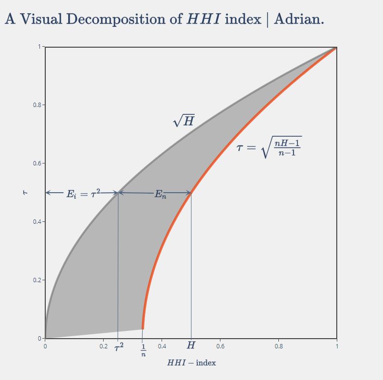
The graph below shows that \(H\) can therefore be decomposed into two components, that is
\[ H = E_i + E_n \]
where \(E_i = \tau^2\), and \(E_n = H-\tau^2\).
We mentioned before that \(\tau\) can be measure of the market concentration resulted from the size distribution (variance) of firms, such that \(E_i=\tau^2\) can be an even better one since it’s smaller than \(H\), which enables us to measure the concentration contributed from the number of firms, measured by \(E_n\).

This decomposition is appealing also in that \(E_n\), from the graph above, effectively is the horizontal difference between the two curves, i.e. the ‘distance’ between the actual market state and the fully competitive market with infinite number of firms (scenario two).
Thus, it’s safe to say this decomposition produces two components explaining the observed market concentration, 1) \(E_i\), the inequality of firm sizes effect, and 2) \(E_n\), the number of firms effect.
Another finding from the graph is that with higher market concentration measured by \(H\), the relative importance of the two components is changing.
When \(H\) is small, most of the concentration is resulted from \(E_n\) as highlighted below, which means the number of firms has a greater impact on market concentration.
When \(H\) is larger, on the other hand, \(E_i\) contributes more to \(H\), which means the firm size inequality plays a bigger role in market concentration.
A potential implication for regulators who are concerned about market concentration, I think, is to 1) focus more on reducing the entry barrier if the current concentration level is moderate, and to 2) focus more on antitrust if the concentration level is already high.
Another implication for researchers is that even though \(H \in [\frac{1}{n}, 1]\) is affected by the number of firms in a market, we should not attempt to use the \(\text{normalized HHI}=\frac{H-1/n}{1-1/n} \in [0,1]\). The reason is now very simple and clear – the normalized HHI is nothing but \(E_i=\tau^2\), which reflects only the market concentration due to the inequality of firm sizes. When we compare across markets or the same market over time, apparently a market with 1,000 firms has a different competitive landscape than a market with only 2 firms.
Acknowledgement
This post is largely a replicate of the paper “A Decomposition of the Herfindahl Index of Concentration” by Giacomo de Gioia in 2017.