AFIN8003 Week 13 - Review

Banking and Financial Intermediation

Dr. Mingze Gao

Department of Applied Finance

2026-11-05

Course overview

About this course

Course description:

• This unit applies finance theory to the context of operational decision-making and risk management in banking and financial intermediation.
• The major decision areas for banking management are covered within a regulatory and corporate responsibility framework.
• Major risks of banks and financial intermediation are being examined.

Key approaches:

• Research-informed teaching.
• Australian focus with global evidence.
• Priority on bank risk management.

Weekly topics

1. Introduction to banking and financial intermediation
2. Risks and regulation
3. Capital management and adequacy
4. Interest rate risk
5. Market risk
6. Credit risk I: individual loan risk
7. Credit risk II: loan portfolio and concentration risk
8. Liquidity risk
9. Liability and liquidity management
10. Sovereign risk, foreign exchange risk, and off-balance-sheet risk
11. Loan sales and securitisation
12. Emerging topics in bank risk management
13. Review

Three big ideas to take with you

Before we walk through twelve weeks of material in one hour, here is the spine of the whole course:

Three big ideas

1. Banks exist because information is costly and trust is scarce. Every risk we have studied — credit, liquidity, market, operational, FX, sovereign — is a price we pay for solving those two problems with leverage.
2. Risk does not disappear; it migrates. Capital regulation moves risk onto buffers. Loan sales move it to buyers. Securitisation moves it to investors. Derivatives move it to counterparties. Open banking and CBDC move it across firms and onto central banks. The exam-ready question is always where did the risk go?
3. The regulator is always one crisis behind. Basel I followed the 1980s loan-loss cycle. Basel III followed the GFC. CPS 230 (operational resilience) followed COVID and cloud incidents. The next rulebook will tell us what just broke.

How to use this review

This deck does not replace the weekly lectures. It is a navigation map. For any concept you are unsure about, jump back to the weekly slides.

The specialness of bank and financial intermediaries

Financial intermediation

A financial system encompasses various financial intermediaries, markets, regulators, and infrastructure in the generation and distribution of financial resources.

Financial intermediation is part of the financial system.

• It is the process by which financial intermediaries, such as banks, facilitate the flow of funds between savers and borrowers.
• Banks are a major part of financial intermediation.

The case for banks

A banking analogue of the Modigliani and Miller (1958) theorem would imply that banks are useless with perfect financial markets.

• In a competitive equilibrium, banks make zero profit and have no impact on other agents’ decisions. Firms are indifferent between bank credit and bonds. (Freixas and Rochet 2023)

The existence of banks (and other financial intermediaries) must be justified by their roles in mitigating market frictions.

• A simple look at the Diamond and Dybvig (1983) model.
• The optimal allocation can be achieved with competitive banks offering deposit contracts and investing in the long-term (i.e., maturity transformation).
  • also, asset transformation, risk transformation and liquidity transformation.
  • Panic-based bank runs may occur even when illiquid assets are risk-free.
• Banks are also better positioned to mitigate informational frictions in the market due to economies of scale.
  • Screening costs in the context of adverse selection (Broecker 1990).
  • Monitoring costs in the context of moral hazard (Holmstrom and Tirole 1997).

Risks and regulation

Bank regulation

Bank failure has large negative externalities — depositor losses, credit-supply collapse, real-economy damage (cf. the GFC). Hence heavy regulation:

• Microprudential — safety and soundness of the individual bank (capital adequacy, risk and liquidity management). The pre-GFC focus.
• Macroprudential — stability of the system (systemic focus, countercyclical policies, stress testing). Added post-GFC.

The two are complementary, not substitutes.

For every risk in this course we apply the I-M-M framework:

1. Identify — definition, source, nature.
2. Measure — gauge exposure.
3. Manage — mitigate.

Capital management and adequacy

Capital management and regulation

The purpose of capital regulation

Bank failures impose costs on people who never agreed to bear them — depositors, borrowers, taxpayers. Capital is the first line of defence that keeps those costs internal to shareholders, not external to the public.

Capital absorbs losses and mitigates insolvency risk. The level a bank holds is guided by:

1. Regulated capital adequacy requirements — country-specific, but the Basel Accords (BCBS of the BIS) provide the global framework.
2. Risk-return trade-offs — capital is expensive; banks won’t hold more than they have to.

From Basel I to Basel III

• Basel I (1988) — first systematic capital adequacy framework; RWA for credit risk only; min Tier 1 = 4%, Total = 8%.
• Basel II (2006) — three pillars (minimum requirements, supervisory review, market discipline); added operational risk; standardized vs IRB.
• Basel 2.5 (2009) — patched market-risk capital after the GFC trading-book disasters.
• Basel III (2010, revised 2017) — our focus. Adds macroprudential layers: buffers, liquidity ratios (LCR/NSFR), leverage ratio, and higher trading-book charges.

Risk-based capital ratio

Under Basel III, depository institutions (DIs) calculate and monitor four capital ratios:

1. Common equity Tier 1 (CET1) risk-based capital ratio \[ \text{CET1 capital ratio} = \frac{\text{CET1 capital}}{\text{Risk-weighted assets}} \tag{1}\]

2. Tier 1 risk-based capital ratio \[ \text{Tier 1 capital ratio} = \frac{\text{Tier 1 capital}}{\text{Risk-weighted assets}} \tag{2}\]

3. Total risk-based capital ratio \[ \text{Total capital ratio} = \frac{\text{Total capital}}{\text{Risk-weighted assets}} \tag{3}\]

4. Tier 1 leverage ratio \[ \text{Tier 1 leverage ratio} = \frac{\text{Tier 1 capital}}{\text{Total exposure}} \tag{4}\]

• The calculation of these capital ratios is complex.
• Use risk-weighted assets (RWA) to distinguish the different credit risks of different assets.
• Measure a DI’s credit risk (on-and off-balance-sheet).

Important

• Additional capital charges for market risk and operational risk.
  • They are summarised below; the unit assesses only RWA for credit risk.

Tiers of capital

• CET1 — common shares, retained earnings, other reserves, minority interests (less regulatory adjustments). The “loss-absorbing-while-going-concern” core.
• Additional Tier 1 — perpetual instruments without maturity (e.g. noncumulative perpetual preferred stock).
• Tier 2 — supplementary capital: subordinated debt, certain loan-loss provisions.

\[\text{Tier 1} = \text{CET1} + \text{Additional Tier 1}, \quad \text{Total Capital} = \text{Tier 1} + \text{Tier 2}\]

Two approaches to measure credit RWA (since Basel II):

• Standardised — used by smaller DIs.
• Internal ratings-based (IRB) — used by large DIs (in Australia, six of the largest banks).

Minimum required capital adequacy ratios

The minimum required capital ratios: \[ \begin{aligned} \text{CET1 capital ratio} &= \frac{\text{CET1 capital}}{\text{Risk-weighted assets}} \ge 4.5\% \\ \text{Tier 1 capital ratio} &= \frac{\text{Tier 1 capital}}{\text{Risk-weighted assets}} \ge 6\% \\ \text{Total capital ratio} &= \frac{\text{Total capital}}{\text{Risk-weighted assets}} \ge 8\% \\ \text{Tier 1 leverage ratio} &= \frac{\text{Tier 1 capital}}{\text{Total exposure}} \ge 3\% \end{aligned} \tag{5}\]

Buffers on top of the minimums

Basel III adds two buffers — both CET1 only — that sit above the minimums:

• Capital conservation buffer: +2.5% of RWA — effective CET1 floor of 7%. If breached, distributions (dividends, bonuses) are restricted.
• Countercyclical capital buffer (CCyB): 0–2.5% of RWA, switched on by national regulators when credit growth is excessive.

The point of the buffers is automatic restraint: as the buffer is eaten, dividend and bonus payouts are choked off before the bank hits the binding minimum.

Risk-based capital: beyond credit risk

So far, the capital ratios (specifically, RWA) are calculated to account for the DI’s credit risk. However, a DI’s insolvency risk can also manifest from interest rate risk, market risk, operational risk, and more.

In Basel III, RWA should be the sum of three components:

1. RWA for credit risk (Week 3)
2. RWA for market risk. Can be calculated using two approaches:¹
   1. Standardized approach proposed by regulators. Revised standards (FRTB) published in 2016 and finalised in 2019.
   2. DI’s internal market risk model subject to regulator approval. Move towards expected shortfall rather than value at risk (VaR).
3. RWA for operational risk. Some complicated calculation.²

Important

The RWA in the minimum capital ratios (Equation 5) is the sum of all three RWAs.

This unit assesses only the RWA for credit risk.

1. For details, see RBC20.9.

2. For details, see RBC20.10.

Interest rate risk

Interest rate risk

Interest Rate Risk

Interest rate risk is the possibility of a financial loss due to changes in interest rates.

One of the key functions performed by financial institutions (especially depository institutions) is maturity transformation. For DIs, they take short-term deposits from depositors and make long-term loans to borrowers. As a result,

1. This maturity transformation means that FIs have mismatches of maturities of their liabilities (e.g., deposits) and assets (e.g., loans).
2. Maturity mismatch exposes FIs to (unexpected) interest rate changes:
   1. refinancing and reinvestment risks
   2. financial instruments have different levels of value sensitivity to interest rate changes
3. Interest rate is volatile and can be unexpected.

Interest rate risk and Basel framework

As discussed previously, the three pillars of Basel framework (since Basel II) include:

1. minimum capital requirements
2. supervisory review
3. effective use of disclosure (for market discipline)

The Pillar 1 involves a capital adequacy framework surrounding minimum ratios of various capital (CET1, Tier 1, Total) to RWA.

• The RWA is sum of RWAs for credit risk, market risk, and operational risk.
• There is currently no “RWA for interest rate risk”.

The Interest Rate Risk in the Banking Book (IRRBB) is part of the Basel capital framework’s Pillar 2 (supervisory review) and Pillar 3 (disclosure).

Repricing model

The repricing (funding-gap) model is a book-value cash-flow analysis of the difference between interest income on assets and interest paid on liabilities over each maturity bucket. APRA requires smaller ADIs to use it for banking-book interest-rate exposure.

Repricing gap = \(RSA - RSL\), where RSA/RSL are rate-sensitive assets/liabilities that reprice within a given maturity bucket (e.g. variable-rate mortgages, term deposits).

\[ \Delta NII_i = GAP_i \times \Delta R_i = (RSA_i - RSL_i) \times \Delta R_i \]

where \(\Delta NII_i\) is the change in net interest income in bucket \(i\).

Duration model

The essence of duration gap model is the concept of duration, which is covered in introductory finance courses.

Duration directly measures the interest rate sensitivity of an asset or liability:

\[ \frac{\Delta P}{P} = - D \times \frac{\Delta R}{1+R} = - MD \times \Delta R \tag{6}\]

where

• \(\Delta P\) is the price change of assets or liabilities
• \(\Delta R\) is the change of interest rate
• \(MD\) is the modified duration that equals to \(\frac{D}{1+R}\)

The larger the numerical value of \(D\), the more sensitive is the price of that asset or liability to changes or shocks in interest rates.

Important

The relationship is only true for small changes in the yield.

Duration and interest rate risk management

Duration can be used to measure a financial institution’s duration gap to evaluate the FI’s overall interest rate exposure. It is possible to calculate the duration of the asset portfolio and of the liability portfolio.

• Duration of a portfolio is the weighted average duration of its components.

Duration of assets portfolio:

\[ D_A = \sum_{i=1}^{N_A} w_{iA} \times D^A_i \]

where \(N_A\) is the total number of assets, \(w_{iA}\) is the market value weight of asset \(i\), \(D^A_i\) is the duration of asset \(i\).

So, change of assets value for a given change in interest rate is

\[ \Delta A = - D_A \times A \times \frac{\Delta R}{1+R} \tag{7}\]

Duration of liabilities portfolio:

\[ D_L = \sum_{i=1}^{N_L} w_{iL} \times D^L_i \]

where \(N_L\) is the total number of liabilities, \(w_{iL}\) is the market value weight of liability \(i\), \(D^L_i\) is the duration of liability \(i\).

So, change of liabilities for a given change in interest rate is

\[ \Delta L = - D_L \times L \times \frac{\Delta R}{1+R} \tag{8}\]

The duration model

Since \(A = L + E\), we have \(\Delta E = \Delta A - \Delta L\). Substituting Equation 7 and Equation 8 and assuming the rate shock is the same on both sides:

\[ \Delta E = - (D_A - D_L k) \times A \times \frac{\Delta R}{1+R} \tag{9}\]

where \(k = L/A\) is leverage. The effect on net worth decomposes into three terms:

1. The leverage-adjusted duration gap \((D_A - D_L k)\).
2. The size of the FI, \(A\).
3. The size of the rate shock, \(\Delta R / (1+R)\).

Market risk

Market risk

Market Risk

Market risk is uncertainty of an FI’s earnings on its trading portfolio caused by changes, particularly extreme changes, in market conditions such as the price of an asset, interest rates, market volatility, and market liquidity.

FIs are concerned about the potential impact of changing market conditions on their trading book and ultimately their net worth and solvency.

A natural question becomes:

How to quantify such impact? What is the potential change in value of trading portfolio for a given period?

More specifically,

1. What is the worst loss we can expect not to exceed with a given confidence level over a specific time horizon?
2. What is the expected loss when losses exceed a certain level over a specific time horizon?

Answering these questions leads to the development of two important concepts for measuring market risk exposure:

1. Value at Risk (VaR).
2. Expected Shortfall (ES).

We start with the concept of Value at Risk (VaR), then discuss its limitations and the use of Expected Shortfall (ES).

Value at Risk (VaR)

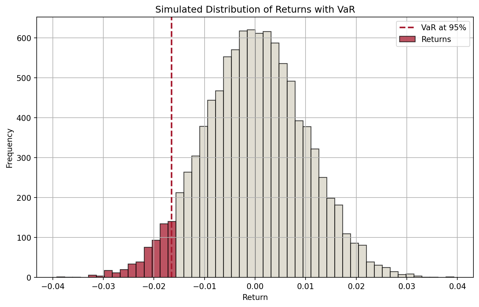
Suppose we know the distribution of an asset’s returns over a specific period (in the future), then for a given confidence level \(c\in[0,1]\) (e.g., \(c=0.95\)), we can partition the distribution into two parts: one (in red) that represents a proportion of \((1-c)\) of the distribution and the other (in blue) accounting the remaining \(c\) proportion.

Figure 1: Distribution of expected returns and VaR

Therefore, the cutoff value of returns that separates the two parts defines:

• a minimum return that we are confident 95% of the time, or
• a maximum loss that we are confident 95% of the time.

Models for computing VaR

Over the years, many models have been developed to compute VaR.

This is because we do not have the return distribution of trading portfolio over a specific period in the future.

• If we do, then VaR is unambiguous.

Therefore, different assumptions lead to different models and approaches. We are interested in three in this course:

1. RiskMetrics (variance-covariance approach)
2. Historic or back simulation
3. Monte Carlo simulation

Expected Shortfall (ES)

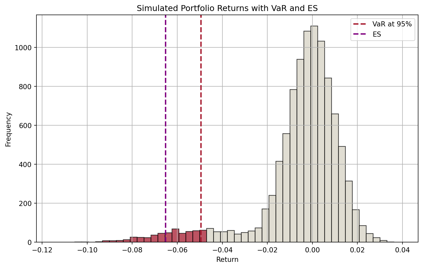
VaR’s drawbacks became evident in the GFC: returns plunged into the fat tail, and VaR projections badly underestimated actual losses. Regulators have since replaced VaR with expected shortfall (ES) — also called “conditional VaR” — the average loss beyond the VaR threshold.

\[ ES(c) = \frac{1}{1-c}\int_c^1 VaR(u)\,du \]

For \(c = 95\%\), ES is the average loss in the worst 5% of outcomes.

Figure 2: Distribution of expected returns and ES

ES: advantages and (potential) problems

ES is the average of losses that occur beyond the VaR level. It provides a better risk assessment by considering the tail of the loss distribution.

In addition, an important advantage of ES over VaR is that ES is subadditive (a coherent risk measure).

• This means that the ES of a portfolio is never greater than the sum of the individual positions’ ESs — consistent with diversification.
• VaR lacks this property: the VaR of a combined portfolio can exceed the sum of the individual VaRs.

Potential issues with the use of ES include:

• Estimation challenges, model dependency, computational complexity.

Credit Risk I: Individual Loan Risk

Credit risk

As suggested by Table 1 below, credit risk is likely the most significant risk factor, the risk that the promised cash flows from loans and securities may not be paid in full (e.g., borrower defaults).

Table 1: RWA of Australian banks in 2024 (source: Capital IQ)

	CBA	Westpac	NAB	ANZ	Macquarie
RWA for credit risk	370,444	351,724	350,891	361,185	98,250
RWA for market risk	52,132	37,510	26,953	30,875	14,277
RWA for operational risk	44,975	48,196	36,102	49,650	17,512
Other RWA	0	0	0	4,872	0
Total RWA	467,551	437,430	413,946	446,582	130,039

Promised vs expected return on a loan

The return on assets approach adjusts for fees, compensating balances, and reserve requirements.

• \(f\) = origination fee; \(b\) = compensating balance share; \(RR\) = reserve requirement; \(BR\) = base rate; \(\phi\) = risk premium.

\[ 1+k = 1+\frac{f+(BR+\phi)}{1-b(1-RR)} \]

Because of default risk, the expected return differs from the promised return. With repayment probability \(p\):

\[ 1+E(r) = p(1+k) + (1-p)\cdot 0 \]

i.e. a probability-weighted average of full repayment (\(1+k\)) and zero recovery.¹

1. In practice, the FI may recover part of the loan (LGD < 100%).

Measurement of credit risk

Many different qualitative and quantitative models are employed to assess the default risk on loans and bonds.

• They are not mutually exclusive.
• An FI manager may use both qualitative and quantitative models and use more than one model to reach a credit decision.

Credit scoring models use observed borrower characteristics to

1. either calculate a score representing the applicant’s default probability, or
2. sort borrowers into different default risk classes.

Scoring models might help to:

• Establish factors that help to explain default risk
• Evaluate the relative importance of these factors
• Improve the pricing of default risk
• Sort out bad loan applicants
• More easily calculate reserve needs

Three broad types

1. Linear probability models
2. Logit models
3. Linear discriminant analysis

Option models of default risk

Rationale:

• A borrower borrows to invest.
• If its investments are successful, the borrower repays.
• If its investments fail and the borrower cannot repay the lender,
  • The borrower has an option to default on its debt, simply turning any remaining assets over to the lender.
• The borrower’s (equity holders’) loss is capped due to limited liability.

Note

The KMV Corporation¹ turned this relatively simple idea into a credit monitoring model.

Many of the largest U.S. FIs are now using this model to determine the expected default frequency (EDF) of large corporations.

1. The KMV Corporation was purchased by Moody’s in 2002 and is now part of Moody’s Analytics Enterprise Risk Solutions.

Credit Risk II: Loan Portfolio and Concentration Risk

Simple models

• Regulations limit exposure to any single borrower.
• As a result, individual loans rarely cause material losses or bank failures.
• Primary cause of credit-related distress is that pools of individual loans sharing similar characteristics perform similarly, especially during extreme conditions.
• An important lesson learned is that products exposed to the same types of risks can have different names and under different business units.

Two simple models widely employed to measure credit risk concentration in the loan portfolio:

1. Migration analysis
2. Concentration limits

Loan portfolio diversification and MPT

MPT can be used to measure and control an FI’s aggregate credit risk exposure.

Any model that seeks to estimate an efficient frontier for loans needs to determine and measure three things:

• The expected return on individual loans
• The risk of individual loans
• The correlation of default risks between loans

The fundamental lesson of MPT is that by taking advantage of its size, an FI can diversify considerable amounts of credit risk as long as the returns on different assets are imperfectly correlated with respect to their default risk adjusted returns.

Moody’s Analytics RiskFrontier Model

Moody’s RiskFrontier applies MPT to the loan portfolio using EDF (from Moody’s Credit Monitor) and LGD as primary inputs — no need for loan returns to be normally distributed.

Three inputs per borrower \(i\):

1. Expected return: \(R_i = AIS_i - (EDF_i \times LGD_i)\), where \(AIS\) is the all-in-drawn spread.¹
2. Unexpected loss (risk): \(\sigma_i = \sqrt{EDF_i(1-EDF_i)} \times LGD_i\), assuming binomial default.²
3. Default correlation \(\rho_{ij}\): estimated from systematic asset-return components of \(i\) and \(j\) via Moody’s Global Correlation Model (GCORR) — a factor model rather than direct historical correlation.

1. In the textbook Saunders et al. (2023), this equation has a typo: \(E(L_i)\) is written as \(R(L_i)\).

2. In the textbook Saunders et al. (2023), this equation is entirely incorrectly written.

Use of derivatives to manage credit risk

• Diversification of loan portfolio helps FIs to manage their credit risk exposure.
• New types of derivative instruments are now available to better allow FIs to hedge their credit risk both on individual loans or on loan portfolios.
  • Credit forwards, options, and swaps.
• These credit derivatives allow FIs to separate the credit risk exposure from the lending process itself.

Credit (default) swaps (CDS)

The most important type of credit derivative.

Why CDS?

1. Credit risk is still more likely to cause an FI to fail than is either interest rate risk or FX risk.
2. CDSs allow FIs to maintain long-term customer lending relationships without bearing the full credit risk exposure from those relationships.

We examine two types of credit swaps:

1. total return swap
2. pure credit swap

Liquidity Risk

Liquidity risk

Liquidity risk is a normal aspect of everyday management of a financial institution (FI). It can arise on both sides of the balance sheet:

• Liability side
  • Depositors and other claim holders decide to cash in their financial claims immediately
    • The DI has to borrow additional funds or sell assets
  • DI need to be able to predict the distribution of net deposit drains
    • The difference between deposit withdrawals and deposit additions on any specific normal banking day

• Asset side
  • Risk from OBS loan commitments and other credit lines
  • Change of the value of investment securities portfolios due to unexpected changes of interest rates
  • Problems associated with ‘quick’ asset sales/fire-sales
    • High costs for turning illiquid assets into cash
    • Low sales price; in worst case, fire-sale price

Managing liquidity — purchased vs stored

Purchased liquidity — buy funds in the market.

• Cash market, repos, wholesale CDs, note/bond issuance.
• Higher rates than deposits, but no asset disposal.
• Disappears in stress.

Stored liquidity — liquidate assets.

• Cash reserves at the central bank, in vaults.
• U.S. Fed reserve requirement reduced to 0% on 26 Mar 2020.
• The RBA imposes no formal reserve requirement.

Liquidity Coverage Ratio (LCR)

Post-GFC, the BCBS introduced two new minimum liquidity standards: LCR (short-term, since Jan 2015) and NSFR (structural, since Jan 2018). Both apply to internationally active banks above size thresholds.

The LCR ensures a DI holds enough high-quality liquid assets (HQLA) to survive a 30-day stress scenario calibrated on GFC conditions:

\[ \text{LCR} = \frac{\text{Stock of HQLA}}{\text{Total net cash outflows over 30 days}} \ge 100\% \]

Reported monthly.

LCR — HQLA and net outflows

HQLA — assets that stay liquid in stress and are unencumbered. Split into:

• Level 1 (no cap, no haircut): cash, central-bank reserves, high-quality sovereign debt.
• Level 2A (capped at 40%, 15% haircut) and Level 2B (further caps and 25–50% haircuts): eligible corporate debt, covered bonds, certain RMBS and equities.

Net cash outflows over 30 days:

\[\text{Net outflows} = Out - \min(In, 75\% \times Out)\]

Cash flows are computed by applying regulator-set draw-down factors to each asset/liability type.

Net Stable Funding Ratio (NSFR)

NSFR targets structural funding stability over a one-year horizon — reducing reliance on short-term wholesale funding (a key GFC failure mode).

\[ \text{NSFR} = \frac{\text{Available stable funding (ASF)}}{\text{Required stable funding (RSF)}} \ge 100\% \]

• ASF — weighted sum of capital, long-term liabilities, and the stable portion of retail/wholesale deposits.
• RSF — weighted sum of on-balance-sheet assets and OBS exposures, with weights set by liquidity profile.

Reported quarterly since 2018.

Bank runs and safety nets

Abnormal deposit drains can trigger a bank run — fuelled by solvency concerns, contagion from related DIs, or sudden preference shifts. A systemic, contagious run is a bank panic.

The two main insulation devices:

1. Deposit insurance — keeps the typical depositor calm so the run never starts.
2. Lender of last resort — central-bank lending to solvent banks against collateral, so a run does not force fire sales.

Moral hazard, the dark side of safety nets

Both backstops are necessary — and both encourage risk-taking. Deposit insurance lets weak banks bid for deposits at the same rate as strong banks. A generous discount window lets banks economise on costly HQLA. The regulator’s job is to price the insurance and the access so the subsidy doesn’t outrun the public benefit.

Liability and Liquidity Management

Two sources of liquidity

Stored liquidity (asset-side) — historically dominant.

• Cash, central-bank reserves, sovereign securities traded in deep markets.
• Government securities act as secondary buffer reserves.
• Composition shaped by reserve requirements and earnings considerations.

Purchased liquidity (liability-side) — dominant today.

• Interbank market (cash market), repos, wholesale issuance.
• Cheaper in normal times — but evaporates in stress.

The day-to-day game is risk-return trade-off: liquid assets earn less; under-shooting LCR/NSFR triggers charges; over-shooting ties up earning assets. Management of the RBA Exchange Settlement Account (ESA) is at the centre of this.¹

1. RBA pays “cash target rate minus 10 basis points” on ESA balances.

The cash market and the RBA

The cash market is the overnight interbank market where banks lend/borrow ES balances.

• Price of funds = the cash rate (RBA’s policy target).
• Supply of ES balances is set by the RBA’s operations.

Pre-COVID (scarce reserves): the RBA managed ES supply via daily repurchase agreements (repos) to keep the cash rate near target.

Now (ample reserves): banks get as many ES balances as they bid for.

• Weekly open market operation — full-allotment repos at the cash rate target plus 10 bp.
• Standing overnight repo facility — at the cash rate target plus 25 bp.
• ES balances earn the cash rate target minus 10 bp.

Liability-side liquidity and management

Aim: construct a low-cost and low-withdrawal-risk liability portfolio. The two are in tension — low-cost liabilities (demand deposits) have high withdrawal risk; low-withdrawal-risk liabilities (CDs) carry higher cost.

Deposit liabilities

• Cheque accounts / demand deposits
• Savings accounts
• Cash management / investment savings accounts
• Fixed-term deposits
• Negotiable certificates of deposit (NCDs)

Non-deposit liabilities

• Interbank funds, repos
• Covered bonds, bank-accepted bills
• Commercial paper / promissory notes
• Subordinated debt, medium-term notes
• Other long-term borrowings

Sovereign Risk, Foreign Exchange Risk, and Off-Balance-Sheet Risk

Foreign exchange risk

An FI’s overall FX exposure in any given currency can be measured by the net position exposure, which is measured in local currency as

\[ \begin{aligned} \text{Net exposure}_i &= (\text{FX assets}_i - \text{FX liabilities}_i) + (\text{FX bought}_i - \text{FX sold}_i) \\ &=\text{Net foreign assets}_i + \text{Net FX bought}_i \end{aligned} \]

where \(i\) represents the \(i\)th currency.

FX volatility and DEAR

Potential loss in any currency \(i\):

\[ \text{Dollar loss/gain}_i = \text{Net exposure}_i \times \text{Shock to FX rate}_i \]

Greater exposure × greater FX volatility ⇒ greater daily earnings at risk (DEAR).

FX volatility itself reflects shifts in the demand/supply of a currency, often driven by inflation and interest-rate differentials — which leads us to the two parity conditions: PPP (inflation) and IRP (interest rates).

Purchasing Power Parity

Nominal interest rate \(R\) is basically the sum of inflation \(\pi\) and real interest rate \(r\) (the Fisher equation).

For two countries, e.g., Australia (AU) and United States (US), we have:

\[ \begin{aligned} R_{AU} &= r_{AU} + \pi_{AU} \\ R_{US} &= r_{US} + \pi_{US} \end{aligned} \]

Assuming real interest rates are equal across countries: \(r_{AU}=r_{US}\), then

\[ R_{AU} - R_{US} = \pi_{AU} - \pi_{US} \]

That is, the (nominal) interest rate spread between Australia and the United States represents the difference in inflation rates between the two countries.

Important

When inflation rates and/or interest rates change, foreign exchange rates (without government control) should adjust to account for relative differences in the price levels (inflation) between the two countries.

Purchasing Power Parity (PPP) is one theory explaining how this adjustment takes place — built on the law of one price: identical goods should have one price across markets in equilibrium.

In its relative form, PPP says the percentage change in the exchange rate is approximately the inflation gap. For yen per US dollar:

\[ \frac{\Delta S_{\text{¥}/\$}}{S_{\text{¥}/\$}} \approx \pi_{JP} - \pi_{US} \]

Interest Rate Parity

Covered interest rate parity (IRP) compares two risk-free ways to invest A$1 for one year:

1. Deposit it in Australia at \(r_{AUD}\).
2. Buy euros at the spot rate \(S_{AUD/EUR}\), deposit them at \(r_{EUR}\), and sell the euros forward today at \(F_{AUD/EUR}\).

With no arbitrage, both must pay the same:

\[ 1 + r_{AUD} = \frac{(1 + r_{EUR})\,F_{AUD/EUR}}{S_{AUD/EUR}} \quad\Longleftrightarrow\quad F_{AUD/EUR} = S_{AUD/EUR} \times \frac{1 + r_{AUD}}{1 + r_{EUR}} \]

The forward rate is pinned by today’s interest rates, not by a forecast.

Managing FX risk

On-balance-sheet hedging

• Requires duration matching to control exposure to foreign interest rate risk
• A direct match of foreign assets and liabilities can result in positive profits for the FI

Off-balance-sheet hedging

• Uses forwards, futures, options and swaps
• Example: hedging with forwards allows FI to offset uncertainty regarding the future spot rate on a currency

Sovereign risk

• Mismatches in the size and maturities of foreign assets and liabilities expose FIs to FX risk.
• Beyond FX risk, holding assets in a foreign country also exposes FIs to country or sovereign risk.
  • e.g., a foreign corporation may be unable to repay the principal or interest on a loan even if it wants to.
  • the government of the country in which a borrower is headquartered may prohibit or limit debt payments

A sovereign country’s (negative) decisions on its debt obligations or the obligations of its public and private organizations may take two forms: repudiation and restructuring.

1. Debt repudiation
   • An outright cancellation of all a borrower’s current and future foreign debt and equity obligations
2. Debt restructuring
   • Change the contractual terms of a loan, such as maturity and interest payment
   • Most common form of sovereign risk

Off-balance-sheet (OBS) activities

OBS items are contingent assets and liabilities — they shape the future balance sheet and produce positive or negative cash flows. True net worth = market value of on- plus off-balance-sheet activities.

Major types

• Loan commitments — promise to lend up to a stated amount at a given rate.
• Letters of credit — contingent guarantees underwriting a buyer’s performance.
• Derivative contracts — forwards, futures, options, swaps.
• When-issued trading — pre-issuance trades.
• Loans sold with recourse.

Motives for OBS

• Fee income.
• Avoid regulatory costs (reserves, deposit-insurance premiums, capital).

OBS is not just risk-increasing — much of it is hedging (interest-rate, FX) and so reduces insolvency risk. Big, creditworthy banks earn substantial OBS fee income.

Loan Sales and Securitisation

From originate-to-hold to originate-to-distribute

For most of the 20th century, banking followed a simple model: originate-to-hold. A bank made a loan, kept it on its books, and collected interest until maturity.

Today, much lending instead follows the originate-to-distribute model:

1. Make loans.
2. Sell them (loan sales) or repackage them (securitisation).
3. Use the proceeds to originate new loans.

A model with consequences

The originate-to-distribute model fuelled the 2008 global financial crisis: once banks no longer held the loans they originated, their incentive to screen and monitor borrowers collapsed. Subprime mortgages were originated, securitised and sold, yet much of the risk came back to banks through tranches they kept and vehicles they sponsored.

Loan sales

• Credit derivatives reduce credit risk without removing assets from the balance sheet.
• Loan sales transfer ownership (and credit risk) to an outside buyer; the loan leaves the balance sheet.
  • Without recourse — no further FI liability after sale (the dominant practice).
  • With recourse — buyer may put the loan back to the FI under defined conditions.
• Loan sales do not create new securities. Pass-throughs, CMOs and MBBs are products of securitisation.

Types of loan sales

Traditional short-term loan sales

• secured by assets of the borrowing firm
• made to investment-grade borrowers or better
• short term (≤ 90 days)
• yields tied to commercial paper rates
• sold in units of $1 million and up

Leveraged loan sales

• term loans (TLs)
• secured by assets of the borrowing firm (often senior secured)
• long maturity (3–6 years)
• floating-rate, historically tied to LIBOR; since LIBOR ended (sterling in 2021, US dollar in 2023), predominantly SOFR in the U.S. and SONIA in the U.K.
• strong covenant protection in theory — see “covenant-lite” below

Note

The definition of “leveraged loan” is ambiguous: some use spreads (e.g. +125 bps), others use rating (BB+ or lower).

Participation vs assignment, and the “good bank / bad bank” trick

Participation — the buyer is not a party to the original credit agreement. They take only partial control and bear double risk: borrower and selling FI.

Assignment — the more common form. All rights transfer; the buyer has a direct claim on the borrower.

Good bank / bad bank carve-outs are a special kind of loan sale: distressed loans move into a separate unit whose job is to sell them off over time.

Reasons for loan sales

1. Capital relief — sell risky assets to reduce RWA.
2. Liquidity — improve asset-side liquidity.
3. Fee income — origination and servicing fees survive the sale.
4. Reserve requirements — historically a driver; matters less now.

Securitisation

Asset securitisation packages loans into newly created securities — asset-backed securities (ABS) — sold to investors. Two mechanisms, both creating off-balance-sheet subsidiaries:

• Special-purpose vehicle (SPV) — passive; pools loans, issues ABS, ceases when loans mature. Underlying loans belong to the investors.
• Structured investment vehicle (SIV) — active; holds loans and funds itself with short-term commercial paper. Underlying loans belong to the SIV.

The SIV problem

SIVs hold long-term assets funded with short-term paper: maturity transformation without deposit insurance. When asset-backed commercial paper markets froze in 2007, SIVs faced runs, and sponsoring banks took the assets back onto their own balance sheets.

Three major forms of securitisation

1. Pass-through security — fractional ownership in a mortgage pool; principal and interest pass through to investors. Prepayment risk is the headline concern.
2. Collateralised mortgage obligation (CMO) — repackages cash flows into tranches (Class A, B, C…) with a pre-specified prepayment waterfall. Different tranches attract different buyers (short A → DIs; long C → insurers, pension funds).
3. Mortgage-backed bond (MBB) / covered bond — bonds secured by a ring-fenced pool that remains on the bank’s balance sheet. Over-collateralised; the trustee monitors the cover pool.

The MBB deposit-insurance subsidy

By pledging collateral to MBB holders, the FI reduces the assets backing insured depositors — effectively transferring risk to the deposit-insurance scheme. This is why APRA caps Australian covered-bond asset encumbrance at 8% of an ADI’s domestic assets.

CLOs and leveraged loans — the post-GFC story

Securitisation never went away after 2008; it migrated.

• The U.S. leveraged loan market reached about US$1.55 trillion at the end of 2025; the U.S. CLO market exceeds US$1 trillion.
• Around 90% of new leveraged loans are now covenant-lite (Berlin et al. 2020), compared with under 25% pre-crisis.
• CLOs absorb roughly two-thirds of new leveraged-loan issuance — they are the marginal buyer.
• Irani et al. (2021) documents that post-GFC capital regulation pushed risky loans out of banks and into less-regulated non-bank lenders — the rise of shadow banking is partly a regulatory artefact.

Was 2020 the next subprime?

In 2018 the Fed, BoE, IMF and BIS all flagged leveraged-loan CLOs as a systemic risk. COVID-19 was the stress test — CLOs survived, in part because of unprecedented central-bank intervention. Whether they would survive a normal recession is still an open question.

Emerging topics in bank risk management

Changing dynamics

Traditional banks face pressure on every side:

• Global competition with other banks.
• Competition with nonbanks (“shadow banks”) — FinTech firms reduce information asymmetry via big-data screening and AI/ML monitoring, and are less regulated than banks.
• Central bank digital currencies (CBDC) — if households hold CBDC instead of bank deposits, banks lose their cheapest funding source.
• Technology — mobile banking has made deposits more mobile too; runs now happen at the speed of a screenshot.
• Business model — the shift to originate-and-distribute (Week 11) means banks now manufacture and ship credit risk rather than warehouse it.

FinTech and BigTech

• FinTech is older than your phone (telegraph 1866, ATM 1967, SWIFT 1973), but post-GFC regulation and the smartphone produced the modern wave.
• A decade ago the consensus was that FinTechs would eat banks. By 2026 the more accurate view is: incumbents kept the deposit franchise; the contest is over who owns the customer interface.
• BigTech (Apple, Google, Amazon, Meta; Alibaba, Tencent) has pushed mostly into payments and embedded credit — partnering with licensed banks rather than becoming one.
• Neobanks are still banks: to take deposits in Australia they need an ADI licence from APRA. The Restricted ADI pathway (since 2018) lowers the entry barrier.

Generative AI in banking

The wave none of the textbooks anticipated. Since ChatGPT (Nov 2022), banks have moved from cautious pilots to scaled deployment: customer service, code generation, and risk and compliance work such as triaging AML alerts.

New risks to manage

• Hallucination in customer-facing chat = mis-selling exposure.
• Third-party concentration — almost every bank’s GenAI stack runs on Microsoft/OpenAI or AWS Bedrock. That is a systemic concentration of operational dependency.
• APRA CPS 230 (operational resilience, effective July 2025) and CPS 234 (information security) now apply to AI service providers.
• Bias and explainability — AI-assisted credit decisions still need to satisfy responsible-lending obligations.

Open Banking and the Consumer Data Right (CDR)

PSD2 (EU, 2018) was the first regulatory move to open banking. Australia’s equivalent is the Consumer Data Right:

• CDR launched in banking (2020), expanded to energy (2022); non-bank lenders share customer data from November 2026.
• Customers consent to share their data with an accredited firm, for a set purpose and up to 12 months; their bank shares it through a standard API.
• It erodes a bank’s information advantage over its own customers, lowering switching costs. He et al. (2023) show it could leave the industry better off yet borrowers worse off.

Central Bank Digital Currency (CBDC)

A CBDC is a digital form of fiat currency issued by the central bank. Two flavours:

• Retail CBDC — for the public; digital cash.
• Wholesale CBDC — for interbank settlement.

The worry for banks

If households can hold central-bank money directly — risk-free, instantly transferable — why hold uninsured commercial-bank deposits? The fear is a structural outflow of deposits to CBDC, forcing banks into more expensive wholesale funding and shrinking credit supply. Chiu et al. (2023) and Niepelt (2024) show the effect depends on design (interest-bearing? capped? how are reserves recycled?).

CBDCs in 2026

• Live retail CBDCs: the Bahamas, Nigeria and Jamaica, all with modest adoption. China’s e-CNY is the largest pilot; since January 2026 its wallet balances pay interest and sit on banks’ balance sheets.
• In design: the digital euro (possible first issuance in 2029) and the digital pound (no decision yet). The U.S. has ruled out a CBDC by executive order.
• Australia: wholesale first. After the eAUD pilot (2023), the RBA and the Digital Finance CRC ran Project Acacia (2024 to 2026), issuing pilot wholesale CBDC to settle tokenised assets.

Wrap-up

Risk migration this semester

Table 2: Where risk migrates — the unifying theme of the unit

Mechanism	Risk moves from…	…to
Capital regulation (Wk 3)	depositors	shareholders (equity buffers)
Hedging with derivatives (Wk 4/5)	the FI	the counterparty
Loan sales (Wk 11)	originating FI	the buyer (often a non-bank)
Securitisation (Wk 11)	originating FI	ABS/CLO investors
Open banking (Wk 12)	the incumbent bank	whoever the customer authorises
CBDC (Wk 12)	commercial-bank deposit base	the central bank’s balance sheet

Finally…

References

Berlin, Mitchell, Greg Nini, and Edison G. Yu. 2020. “Concentration of Control Rights in Leveraged Loan Syndicates.” Journal of Financial Economics 137 (1): 249–71. https://doi.org/10.1016/j.jfineco.2020.02.002.

Broecker, Thorsten. 1990. “Credit-Worthiness Tests and Interbank Competition.” Econometrica 58 (2): 429.

Chiu, Jonathan, Seyed Mohammadreza Davoodalhosseini, Janet Jiang, and Yu Zhu. 2023. “Bank Market Power and Central Bank Digital Currency: Theory and Quantitative Assessment.” Journal of Political Economy 131 (5): 1213–48. https://doi.org/10.1086/722517.

Diamond, Douglas W., and Philip H. Dybvig. 1983. “Bank Runs, Deposit Insurance, and Liquidity.” Journal of Political Economy 91 (3): 401–19.

Freixas, Xavier, and Jean-Charles Rochet. 2023. Microeconomics of Banking. 3rd ed. MIT Press.

He, Zhiguo, Jing Huang, and Jidong Zhou. 2023. “Open Banking: Credit Market Competition When Borrowers Own the Data.” Journal of Financial Economics 147 (2): 449–74. https://doi.org/10.1016/j.jfineco.2022.12.003.

Holmstrom, Bengt, and Jean Tirole. 1997. “Financial Intermediation, Loanable Funds, and the Real Sector.” Quarterly Journal of Economics 112 (3): 663–91.

Irani, Rustom M, Rajkamal Iyer, Ralf R Meisenzahl, and José-Luis Peydró. 2021. “The Rise of Shadow Banking: Evidence from Capital Regulation.” The Review of Financial Studies 34 (5): 2181–235. https://doi.org/10.1093/rfs/hhaa106.

Modigliani, F, and M H Miller. 1958. “The Cost of Capital, Corporation Finance and the Theory of Investment.” The American Economic Review 48 (3): 261–97.

Niepelt, Dirk. 2024. “Money and Banking with Reserves and CBDC.” The Journal of Finance 79 (4): 2505–52. https://doi.org/https://doi.org/10.1111/jofi.13357.

Saunders, Anthony, Marcia Millon Cornett, and Otgo Erhemjamts. 2023. Financial Institutions Management ISE. 11th ed. McGraw Hill.