In 48 hours, the 16th-largest bank in the United States was seized by regulators. Depositors withdrew $42 billion in a single day. The cause? Not fraud. Not bad loans. Interest rate risk.
SVB had loaded up on long-duration bonds when rates were near zero. When the Fed raised rates by over 4 percentage points in 2022, the market value of those bonds plummeted — wiping out nearly all of SVB’s equity.
We will return to SVB throughout this lecture. By the end, you will be able to quantify exactly how exposed SVB was — and why it collapsed.
What is interest rate risk?
Interest Rate Risk
Interest rate risk is the possibility of a financial loss due to changes in interest rates.
Recall that in Week 1, we explained one of the key functions performed by financial institutions (especially depositary institutions) is maturity transformation. For DIs, they take short-term deposits from depositors and make long-term loans to borrowers.
Table 1: Typical balance sheet of a DI
Assets
Liabilities and Equity
Loans (relatively long-term)
Deposits (relatively short-term)
Other assets
Other liabilities
Equity
As a result,
This maturity transformation means that FIs have mismatches of maturities of their liabilities (e.g., deposits) and assets (e.g., loans).
Maturity mismatch exposes FIs to (unexpected) interest rate changes:
refinancing and reinvestment risks
financial instruments have different levels of value sensitivity to interest rate changes
Interest rate is volatile and can be unexpected.
Maturity mismatch: refinancing risk
Consider an example bank that has $2 million of 10-year fixed-rate loans and $1 million of 1-year fixed-rate term deposits now. The bank expects to have the same balance sheet in the future.
What would happen in 1 year from now?
Term deposits mature. Some deposits may be withdrawn.
In this case, the bank needs to take additional deposits to maintain the size of balance sheet.
However, the interest rate (deposit rate) could be higher in the future, which means higher costs for the bank.
This is a typical refinancing risk — the costs of rolling over or re-borrowing funds rise above the returns generated on investments.
Tip
Think of this like a homeowner on a variable-rate mortgage when the RBA hikes rates: your repayments go up but your income (asset) stays the same.
Maturity mismatch: reinvestment risk
Consider another example bank that has $2 million of 1-year fixed-rate loans and $1 million of 2-year fixed-rate term deposits now. The bank expects to have the same balance sheet in the future.
What would happen in 1 year from now?
Loans mature.
In this case, the bank needs to reinvest into some other assets (e.g., make loans).
However, the interest rate (on the loan) could be lower in the future, which means reduced returns for the bank.
This is a typical reinvestment risk — the returns on funds to be reinvested fall below the cost of funds.
Tip
The flip side: imagine a retiree reinvesting maturing term deposits when rates have fallen. Their income drops even though their cost of living hasn’t.
Financial instruments’ value sensitivity to interest rate
The value of longer-maturity instruments typically is more sensitive to interest rate.
For example, a bond’s price is given by
\[
P = \sum_{t=1}^T\frac{C}{(1+r)^t} + \frac{F}{(1+r)^T}
\tag{1}\]
where \(C\) is coupon payment, \(F\) face value, \(T\) maturity, and \(r\) interest rate.
If a FI is financed by issuing long-term bonds and invests in short-term loans, given a change in interest rate, its liabilities’ value would change by more than the change in its assets’ value, thereby causing an impact on its net worth.
Code
viewof maturity4 = Inputs.range( [1,30], {value:15,step:1,label:"Maturity (years):"})viewof couponRate4 = Inputs.range( [0.01,0.2], {value:0.05,step:0.01,label:"Coupon rate:"})d = {const f =100;let c, m; c = couponRate4; m = maturity4;functionpv(c, f, t, r) {return c * (1- (1+r)**(-t)) / r + f / (1+r)**(t) }const prices = {"YTM": [],"Price": []};let coupon = f * c;for (let ytm =0.01; ytm <20; ytm++) {let price =pv(coupon, f, m, ytm/100); prices["YTM"].push(ytm); prices["Price"].push(price); }return prices;}data4 =transpose(d)Plot.plot({caption:"Assume $100 bond, annual coupons paid in arrears and effective annual discount rate.",x: {padding:0.4,label:"YTM (%)"},grid:true,marks: [ Plot.ruleY([0,100]), Plot.ruleX([0]), Plot.lineY(data4, {x:"YTM",y:"Price",stroke:"blue"}), ]})
The level and movement of interest rates
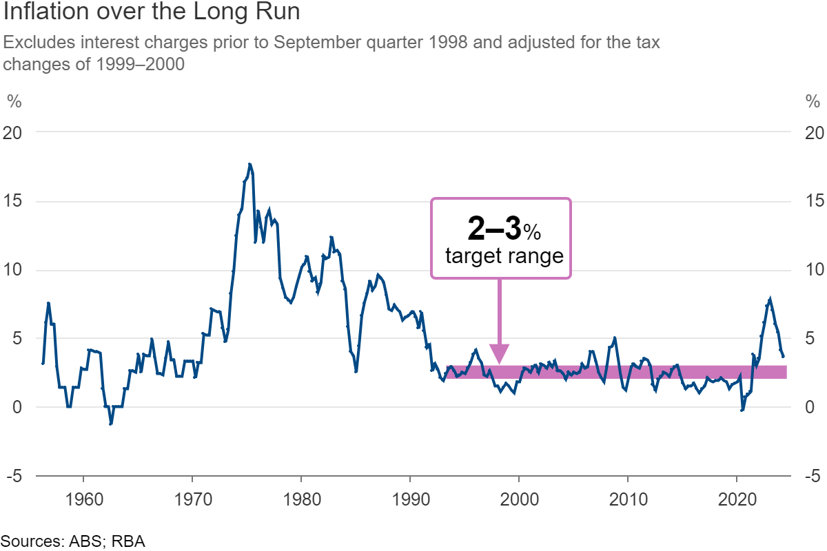
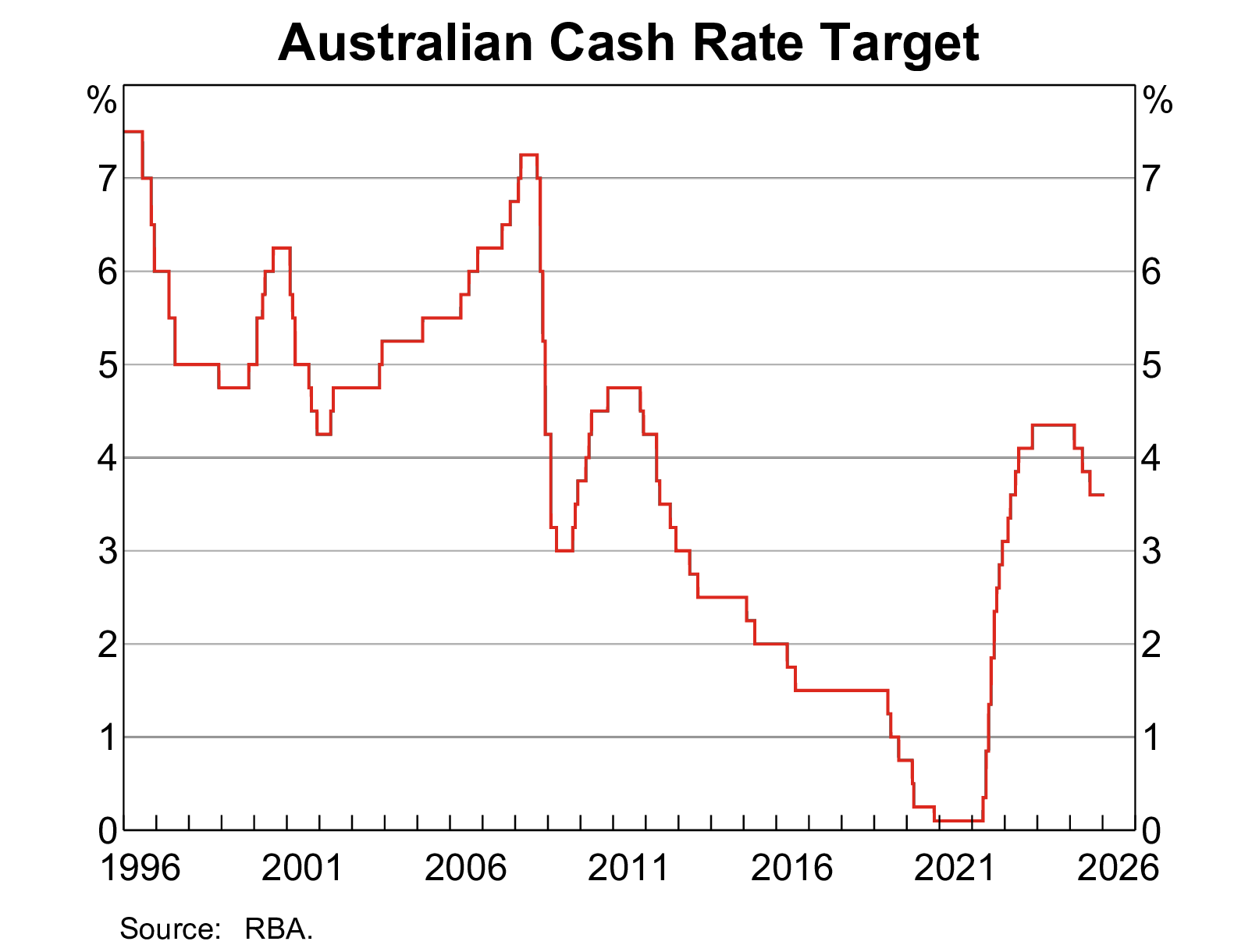
The degree of interest rate volatility is directly linked to the monetary policy of the Reserve Bank of Australia (RBA).
The RBA targets an inflation band of 2–3% per annum (in place since 1993) and uses the cash rate as its primary instrument.
When the economy is running hot, the RBA raises the cash rate — which flows through to every loan and deposit rate in the system.
Conversely, in downturns (such as COVID), the RBA cuts rates to near zero.
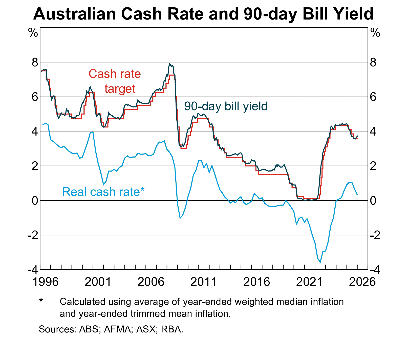
These shifts in the policy stance — particularly when they are large and fast — generate significant interest rate volatility across the financial system.
Figure 3: Australian cash rate target and 90-day bill yield
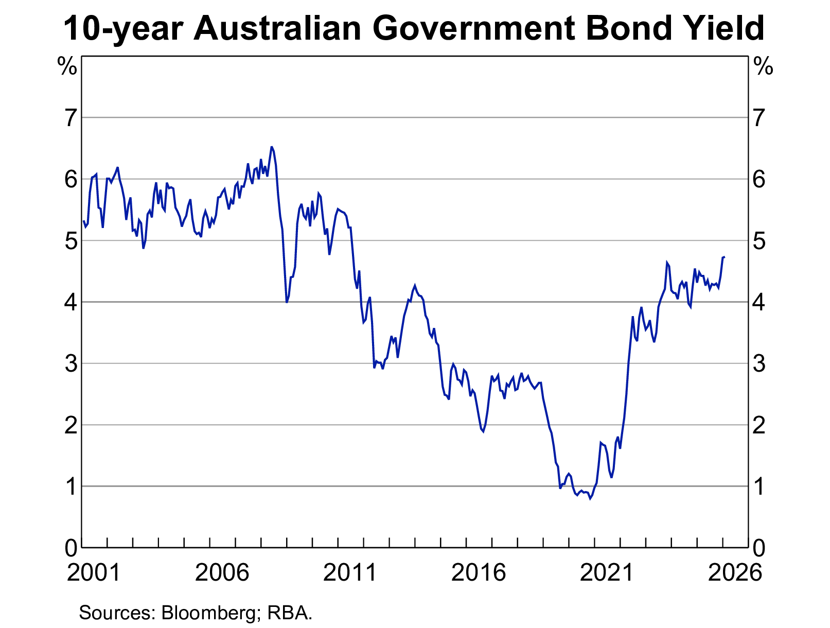
The level and movement of interest rates
Figure 4: 10-year Australian government bond yield
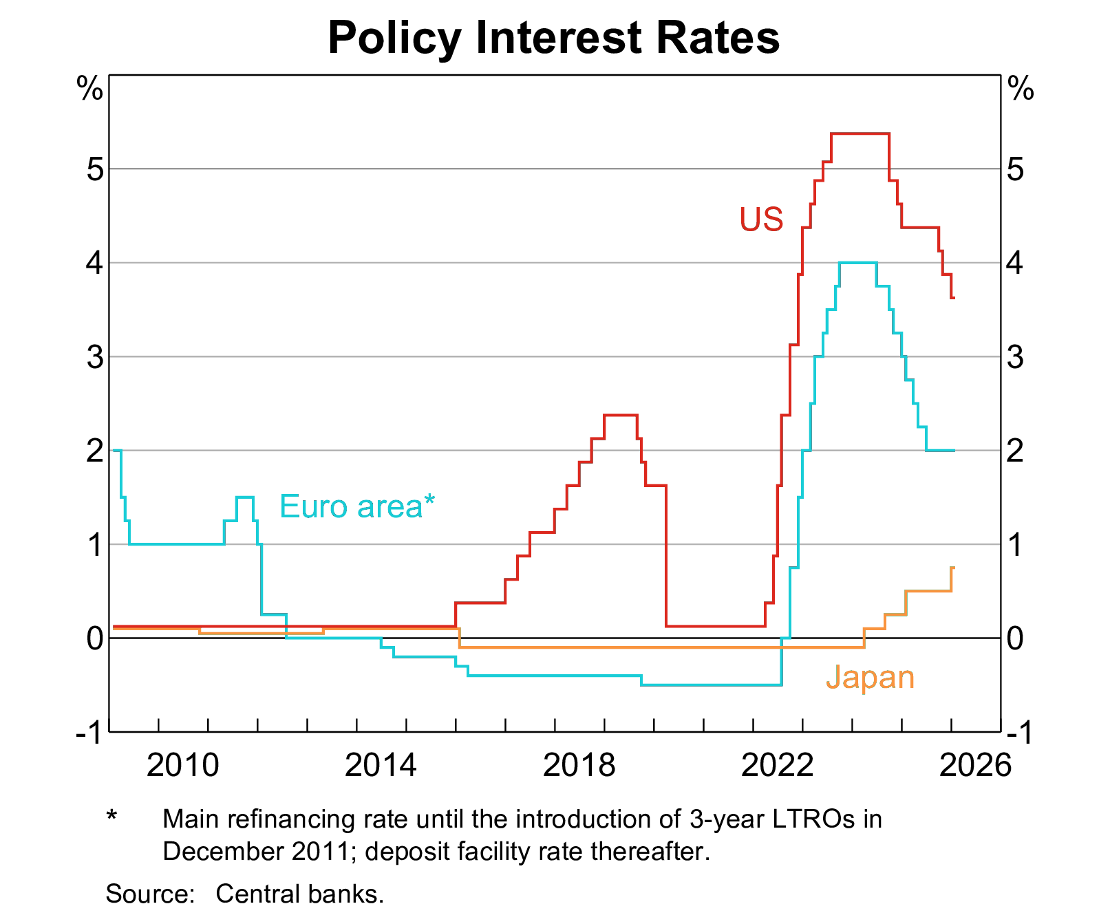
Figure 5: Policy interest rates
Important
Notice the 2022–23 hiking cycle: the US Fed raised rates by over 500 basis points in 18 months — the fastest tightening in 40 years. This is the macroeconomic backdrop for the SVB collapse.
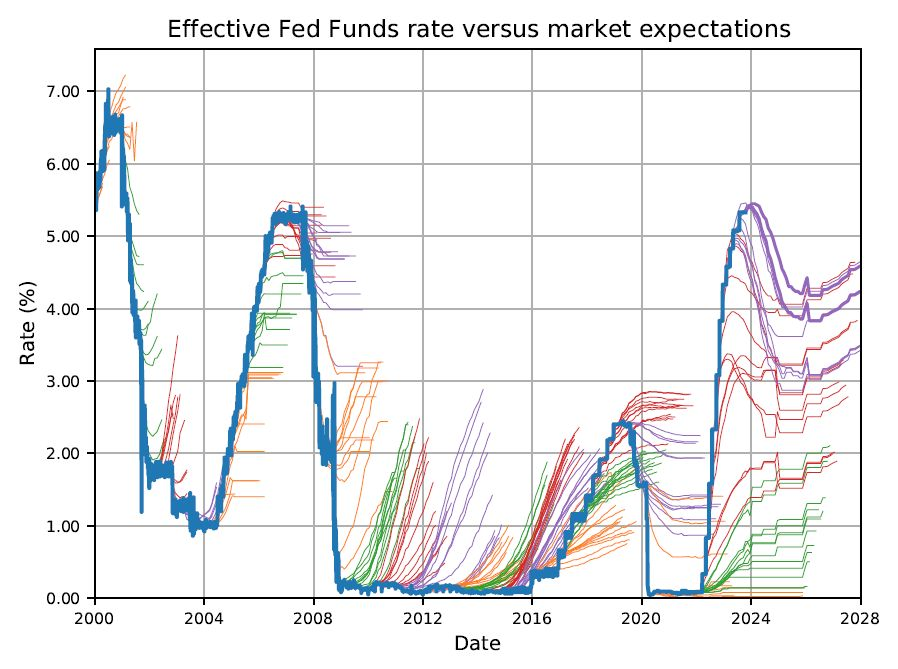
The market is bad at guessing interest rates
Figure 6: The market does not always correctly forecast interest rates
SVB’s own risk models assumed rates would stay low. So did the market. This is precisely why managing — not just forecasting — interest rate risk matters.
Interest rate risk and Basel framework
As discussed last week, the three pillars of Basel framework (since Basel II) include:
minimum capital requirements
supervisory review
effective use of disclosure (for market discipline)
The Pillar 1 involves a capital adequacy framework surrounding minimum ratios of various capital (CET1, Tier 1, Total) to RWA.
The RWA is sum of RWAs for credit risk, market risk, and operational risk.
There is currently no “RWA for interest rate risk”.
The Interest Rate Risk in the Banking Book (IRRBB) is part of the Basel capital framework’s Pillar 2 (and Pillar 3).
Interest rate risk and Basel framework (cont’d)
Basel III guidelines address the issue of interest rate risk primarily through:
Interest Rate Risk in the Banking Book (IRRBB)
Banks are required to identify, measure, monitor, and control IRRBB. This involves regular stress testing, scenario analysis, and the application of appropriate capital charges to cover potential losses from adverse interest rate movements.
Basel III mandates regular stress testing to evaluate the impact of significant changes in interest rates on a bank’s earnings and capital.
Supervisory Review Process (Pillar 2)
Under Pillar 2, banks are required to conduct internal assessments of their capital adequacy in relation to their risk profile, including IRRBB. Supervisors review these assessments to ensure adequate management.
Disclosure Requirements (Pillar 3)
Under Pillar 3, Basel III enhances transparency by requiring banks to disclose their exposure to interest rate risk. This includes detailed reporting on the impact of interest rate changes on earnings and economic value.
Warning
SVB was exempt from enhanced IRRBB stress testing requirements under US rules — a regulatory gap that regulators have since moved to close.
Measuring interest rate risk
An overview
From here, we study specific models and techniques for measuring an FI’s interest rate risk. But first, let’s establish the general framework.
To measure interest rate risk, we need to specify:
Which FI characteristic are we concerned about? Income? Net worth? Something else?
How sensitive is that characteristic to interest rate changes?
What is the potential size of the rate move?
Are we using book value or market value?
What time frame are we considering?
Why does the choice of measure matter?
A bank can look perfectly healthy on a book-value basis while being technically insolvent on a market-value basis. SVB’s held-to-maturity (HTM) portfolio was carried at amortised cost — but its fair value had fallen by $15 billion.
Interest rate risk models
The rest of this lecture discusses two models for measuring interest rate risk with different focuses.
Table 2: A simple comparison of two interest rate risk models
Repricing model
Duration model
Which characteristic?
Net interest income (NII)
Net worth
Sensitivity measurement?
By assumption
Duration
Size of risk?
Flexible
Flexible
Book value or market value?
Book value
Market value
Time frame?
Flexible
Flexible
Note
The repricing model would have shown SVB as a concern (rising deposit costs). The duration model would have screamed alarm — it accounts for the market value collapse of its long-duration bond portfolio.
Repricing model
The repricing model
Repricing model is also known as the funding gap model.
A book value accounting cash flow analysis of the repricing gap between the interest income earned on an FI’s assets and the interest paid on its liabilities over some period.
Focus on the changes of net interest income (NII).
A simple model used by small FIs.
APRA requires smaller ADIs to use the repricing method to estimate interest rate exposures in their banking book for capital adequacy purposes.
A revised reporting standard (ARS 117.0) was completed in July 2024 and became effective in 2025.1
Repricing gap, RSA and RSL
Repricing gap is the difference between rate-sensitive assets (RSA) and rate-sensitive liabilities (RSL).
RSA: assets whose interest rates will be repriced or changed over some future period (rate-sensitive assets)
RSL: liabilities whose interest rates will be repriced or changed over some future period (rate-sensitive liabilities)
An asset (or liability) is “rate-sensitive” if it is repriced at or near current market interest rates within a certain time horizon (or maturity bucket). For example,
a variable-rate mortgage’s interest rate may be reset every quarter based on the prevailing interest rate.
interest rate of term deposits are also adjusted frequently.1
Maturity (Tenor) buckets
Under repricing model, banks report their repricing gaps for various maturity buckets. For example,
One day (overnight).
More than 1 day to 3 months.
More than 3 months to 6 months.
More than 6 months to 12 months.
More than 1 year to 5 years.
More than 5 years.
How to determine RSA/RSL for each bucket?
Ask a simple question: Will or can this asset or liability have its interest rate changed within the maturity bucket? If yes → rate-sensitive. If no → not rate sensitive.
Maturity buckets and RSA/RSL
Let’s practice. Try to identify the one-year RSA and RSL given the following assets and liabilities of a bank.
Assets:
Liabilities:
Repricing gaps
Table 3: Repricing gaps ($ millions)
Assets
Liabilities
Gaps
Cumulative gap
1
One day
20
30
-10
-10
2
One day to three months
30
40
-10
-20
3
Three months to six months
70
85
-15
-35
4
Six months to 12 months
90
70
+20
-15
5
One year to five years
40
30
+10
-5
6
Over five years
10
5
+5
0
Total
$260
$260
For example, a negative $10 million difference between RSA and RSL repriced in one day. A rise in the overnight rate would lower the FI’s net interest income since the FI has more rate-sensitive liabilities than assets in this bucket.
The repricing model
The repricing model estimates the change in the FI’s net interest income in a particular repricing bucket if interest rates change.
\(\Delta NII_i\) is the change in net interest income in the \(i\)th bucket.
\(GAP_i\) is the dollar size of the gap between the book value of RSA and RSL in maturity bucket \(i\).
\(\Delta R_i\) is the change in the level of interest rates impacting assets and liabilities in the \(i\)th bucket.
The repricing model: examples
One-day repricing gap
In the first bucket of Table 3, if the gap is negative $10 million and overnight interest rate rises by 1 percent, the annualised change in the FI’s future NII is:
So, the repricing model suggests a loss of $100,000 in net interest income for the FI.
One-year (cumulative) repricing gap
The one-year cumulative repricing gap is −$15 million from Table 3.
\[
\Delta NII = CGAP \times \Delta R = -\$15M \times 0.01 = -\$150,000
\]
If the average interest rate rises by 1 percent, the model suggests a loss of $150,000 in net interest income.
The repricing model: examples
Assume both RSAs and RSLs equal $155 million. Suppose that there is a general interest rate rise and that the rates on RSAs rise by 1.2 percent and rates on RSLs rise by only 1 percent. What is the resulting change in NII?
Check Item 7A. Quantitative and qualitative disclosure about market risk.
The repricing model: problems
The repricing model is simple and intuitive, but is NOT an accurate measure of interest rate risk.
Major shortcomings:
It is over-aggregative.
It ignores the market value effects of interest rate changes: it focuses on income and ignores capital gains/losses.
It uses the banking book and hence book values of assets and liabilities.
It fails to deal with the problem of rate-insensitive asset and liability runoffs and prepayments.
It ignores cash flows from off-balance-sheet activities.
Warning
SVB reported a manageable repricing gap for its short-term NII. But the repricing model completely missed the $15 billion hole in the market value of its bond portfolio. This is exactly why regulators push larger banks towards market-value-based models.
Duration model
Motivation
In the early 2000s, the BIS issued a consultative document suggesting a standardised model be used by regulators to evaluate a bank’s interest rate risk exposure. The approach suggested is firmly based on market value accounting and the duration gap model.
The duration gap model:
considers market values and the maturity distributions of an FI’s assets and liabilities.
considers the degree of leverage on an FI’s balance sheet.
considers the timing of the payment or arrival of cash flows on assets and liabilities.
is a more comprehensive measure of an FI’s interest rate risk.
Bigger banks have adopted the duration model as their primary measure of interest rate risk.1
Duration
The essence of the duration gap model is the concept of duration, which is covered in introductory finance courses.
Simply put, duration is the weighted-average time to maturity on the loan using the relative present values of the cash flows as weights.
\[
D = \sum_{t=1}^{N} w_t \times t
\]
where \(D\) is the duration, and
\[
w_t = \frac{\text{PV of the cash flow at time } t}{\text{Total PV of all cash flows}}
\]
Tip
Intuition: duration is the “centre of gravity” of a bond’s cash flows. A long-maturity bond has a high duration — its cash flows sit far in the future, so their present value is very sensitive to the discount rate.
Duration: example
Consider the duration of a 3-year coupon bond with a face value of $1,000, a coupon rate of 5%, and a yield to maturity of 4%. The bond pays annual coupons.
Code
import pandas as pd# Parametersface_value, coupon_rate, yield_to_maturity, years =1000, 0.05, 0.04, 3annual_coupon_payment = face_value * coupon_rate# Initialize and calculate valuesdata = [ (t, annual_coupon_payment if t < years else annual_coupon_payment + face_value)for t inrange(1, years +1)]total_pv =sum(payment / (1+ yield_to_maturity) ** t for t, payment in data)table = [ ( t, payment, pv := payment / (1+ yield_to_maturity) ** t, weight := pv / total_pv, t * weight, )for t, payment in data]# Create DataFramedf = pd.DataFrame( table, columns=["Time (Years)","Payment ($)","PV of Payment ($)","Weight (PV/Total PV)","Weighted Time", ],)# Add totals rowtotals = df.sum(numeric_only=True)totals = pd.DataFrame(totals).Ttotals["Time (Years)"] ="Total"df = pd.concat([df, totals], ignore_index=True)df.style.highlight_max(["Weighted Time"]).format(precision=2).hide()
Table 4: Calculating the duration of a 3-year bond
Time (Years)
Payment ($)
PV of Payment ($)
Weight (PV/Total PV)
Weighted Time
1
50.00
48.08
0.05
0.05
2
50.00
46.23
0.04
0.09
3
1050.00
933.45
0.91
2.72
Total
1150.00
1027.75
1.00
2.86
The bond’s duration is 2.86 years.
Duration: another example
Consider the duration of a 5-year coupon bond with a face value of $1,000, a coupon rate of 4%, and a yield to maturity of 6%. The bond pays annual coupons.
Code
import pandas as pd# Parametersface_value, coupon_rate, yield_to_maturity, years =1000, 0.04, 0.06, 5annual_coupon_payment = face_value * coupon_rate# Initialize and calculate valuesdata = [ (t, annual_coupon_payment if t < years else annual_coupon_payment + face_value)for t inrange(1, years +1)]total_pv =sum(payment / (1+ yield_to_maturity) ** t for t, payment in data)table = [ ( t, payment, pv := payment / (1+ yield_to_maturity) ** t, weight := pv / total_pv, t * weight, )for t, payment in data]# Create DataFramedf = pd.DataFrame( table, columns=["Time (Years)","Payment ($)","PV of Payment ($)","Weight (PV/Total PV)","Weighted Time", ],)# Add totals rowtotals = df.sum(numeric_only=True)totals = pd.DataFrame(totals).Ttotals["Time (Years)"] ="Total"df = pd.concat([df, totals], ignore_index=True)df.style.highlight_max(["Weighted Time"]).format(precision=2).hide()
Table 5: Calculating the duration of a 5-year bond
Time (Years)
Payment ($)
PV of Payment ($)
Weight (PV/Total PV)
Weighted Time
1
40.00
37.74
0.04
0.04
2
40.00
35.60
0.04
0.08
3
40.00
33.58
0.04
0.11
4
40.00
31.68
0.03
0.14
5
1040.00
777.15
0.85
4.24
Total
1200.00
915.75
1.00
4.61
The bond’s duration is 4.61 years. Note: coupon < YTM, so the bond trades at a discount — market price ≈ $915.73, not $1,000.
The economic meaning of duration
We are interested in the sensitivity of bond price to interest rate.
That is, how much the price of a bond changes when the interest changes.
Duration directly measures the interest rate sensitivity of an asset or liability:
\[
\frac{\Delta P}{P} = - D \times \frac{\Delta R}{1+R} = - MD \times \Delta R
\tag{2}\]
where
\(\Delta P\) is the price change of assets or liabilities
\(\Delta R\) is the change of interest rate
\(MD\) is the modified duration that equals to \(\frac{D}{1+R}\)
The larger the numerical value of \(D\), the more sensitive is the price of that asset or liability to changes or shocks in interest rates.
Important
The relationship is only true for small changes in the yield.
The economic meaning of duration
Why does it work?
\[
\frac{\Delta P}{P} = - D \times \frac{\Delta R}{1+R} = - MD \times \Delta R
\]
We can write out the price formula of a bond and take its partial derivative with respect to yield.
Why is it only true for small changes in the yield?
Because duration also changes as yield changes.
We assumed the duration is constant given a small \(\Delta R\).
Duration and price changes: example
Consider the previous example of a 5-year annual-coupon bond in Table 5 with a 4% coupon rate and 6% yield. It has a duration of 4.61 years and a market price of $915.73.
What is the price change if the interest rate (yield) decreases by 1 percent (\(\Delta R=-0.01\))?
Note
Recall Equation 2 that \(\frac{\Delta P}{P} = - D \times \frac{\Delta R}{1+R} = - MD \times \Delta R\).
\[
\Delta P = - MD \times P \times \Delta R = - 4.349 \times \$915.73 \times (-0.01) \approx +\$39.82
\]
That is, a one percentage point (100 basis points) decrease in yield would increase bond price by approximately $39.82.
Note that \(MD\times P\) is also called “dollar duration” — the dollar sensitivity per unit change in yield.
Features of duration
Duration increases with the maturity of a fixed-income security, but at a decreasing rate.
Duration decreases as the yield on a security increases.
Duration decreases as the coupon or interest payment increases.
Duration and interest rate risk management
Now that we have refreshed our knowledge of duration, how is duration relevant in FI’s interest rate risk management?
Let’s consider two cases.
A single security.
A portfolio of securities (e.g., the balance sheet).
Duration and interest rate risk management: single security
Superannuation funds or insurers often have to make a specific amount of payment to their policyholders at a given future date. How to guarantee it? Investments may decrease in value if interest rate changes over the period.
There are two options:
Buy a zero-coupon bond which matures exactly when the payment is made in the future.
Buy bond(s) with a duration that matches the payment date.1
However,
Option 1 is very difficult because there simply may not be any such zero-coupon bonds with desirable maturities.
Option 2 is manageable and practical!
Duration and interest rate risk management: balance sheet
Duration can be used to measure a financial institution’s duration gap to evaluate the FI’s overall interest rate exposure. It is possible to calculate the duration of the asset portfolio and of the liability portfolio.
Duration of a portfolio is the weighted average duration of its components.
Duration of assets portfolio:
\[
D_A = \sum_{i=1}^{N_A} w_{iA} \times D^A_i
\]
where \(N_A\) is the total number of assets, \(w_{iA}\) is the market value weight of asset \(i\), \(D^A_i\) is the duration of asset \(i\).
So, change of assets value for a given change in interest rate is
\[
\Delta A = - D_A \times A \times \frac{\Delta R}{1+R}
\tag{3}\]
Duration of liabilities portfolio:
\[
D_L = \sum_{i=1}^{N_L} w_{iL} \times D^L_i
\]
where \(N_L\) is the total number of liabilities, \(w_{iL}\) is the market value weight of liability \(i\), \(D^L_i\) is the duration of liability \(i\).
So, change of liabilities for a given change in interest rate is
\[
\Delta L = - D_L \times L \times \frac{\Delta R}{1+R}
\tag{4}\]
The duration model
We know that total assets (\(A\)) is the sum of liabilities (\(L\)) and equity (\(E\)): \(A=E+L\).
Therefore, \(E = A - L\), and \(\Delta E = \Delta A - \Delta L\).
\[
\Delta E = - (D_A - D_L k) \times A \times \frac{\Delta R}{1+R}
\]
The effect of interest rate changes on the market value of an FI’s net worth breaks down into three effects:
The leverage-adjusted duration gap: \((D_A-D_L k)\)
The size of the FI: \(A\)
The size of the interest rate shock: \(\frac{\Delta R}{1+R}\)
The duration model: example
Suppose a FI has total assets of $100 million and total liabilities of $90 million.
Assume that the average duration of assets is 5 years, while the average duration of liabilities is 3 years. The current interest rate is 10%, but is expected to increase to 11% in the future.
We can calculate the expected change in the FI’s net worth as follows:
This means that the FI could lose $2.09 million in net worth if interest rates rose by 1 per cent.
How can the FI manage the interest rate exposure?
Reduce \(D_A\), and/or
Increase \(D_L\), and/or
Increase leverage \(k\), and/or
…
Case study: applying the duration model to SVB
Let’s return to Silicon Valley Bank. Here is a stylised version of its end-2022 balance sheet:
Stylised SVB balance sheet, end of 2022
Item
Amount
Approx. Duration
HTM investment securities (MBS & Treasuries)
$91.3B
~5.6 years
AFS investment securities
$26.1B
~3.6 years
Loans and other assets
$94.4B
~2.0 years
Total assets
$211.8B
Deposits (mostly demand)
$173.1B
~0.2 years
Other liabilities
$22.7B
~1.0 years
Equity
$16.0B
The duration gap was enormous
Estimated \(D_A \approx 3.6\) years, \(D_L \approx 0.3\) years, \(k = L/A \approx 0.92\).
Leverage-adjusted duration gap \(= D_A - D_L \times k \approx 3.6 - 0.3 \times 0.92 \approx 3.3\) years.
With a 3% rise in rates: \(\Delta E \approx -(3.3) \times \$211.8B \times \frac{0.03}{1.01} \approx -\$20.8B\).
SVB had only $16B in equity. The model predicted insolvency.
SVB: what regulators missed — and what the model revealed
The repricing model showed manageable NII effects (deposits were largely non-interest-bearing demand deposits — not rate-sensitive in the short run).
But the duration model told a very different story:
\(D_A \gg D_L\): assets were long-duration bonds, liabilities were short-duration deposits.
A massive positive duration gap meant that rising rates would destroy equity value.
By end of 2022, the HTM portfolio alone had $15.1B in unrealised losses — equivalent to 94% of SVB’s equity.
SVB’s management chose to hold bonds as HTM (avoiding mark-to-market losses on paper). But the economic loss was real.
Key lesson
Book-value accounting can hide market-value insolvency. The duration gap model, based on market values, would have sounded the alarm years earlier.
Regulatory gap
SVB was exempted from enhanced stress testing for IRRBB under US rules for banks with assets below $250B. Following the collapse, US regulators have proposed extending these requirements to banks above $100B.
Immunization and regulatory considerations
Regulators, like APRA in Australia, require banks to hold a minimum amount of capital against their (risk-weighted) assets.
Thus, in order to comply with regulations, the aim of risk management should not be \(\Delta E=0\) but \(\Delta \left(\frac{E}{A}\right) = 0\).
Instead of setting \(D_A-D_L k=0\), the bank now needs to target \(D_A-D_L=0\).
Difficulties in applying duration model
Duration matching can be costly.
Immunization is a dynamic problem — duration changes as time passes and as rates change, so a bank must continuously rebalance.
Large interest rate changes can happen (and the linear approximation breaks down).
Convexity — a second-order correction that matters for large rate moves.
Note
Had SVB actively managed its duration gap — for example, by using interest rate swaps to pay fixed / receive floating — it could have hedged much of its exposure without selling the bonds. This is what most large banks do.