AFIN8003 Week 8 - Credit Risk II: Loan Portfolio and Concentration Risk

Banking and Financial Intermediation

Dr. Mingze Gao

Department of Applied Finance

2024-09-11

Credit Risk II: Loan Portfolio and Concentration Risk

Introduction

  • In Week 6, we discussed alternative ways by which FI managers can measure the default (credit) risk on individual loans.
  • FIs typically hold a portfolio of loans and hence credit risk should also be measured and managed in a portfolio context.
  • This week, we discuss several models used by FI managers to assess the risk of the overall loan portfolio.
  • We will also discuss the use of derivatives to manage credit risk.

Simple models of loan concentration risk

Simple models

Caution

A large credit risk exposure to a single borrower or group of related borrowers poses a potential threat to a bank’s safety and soundness.

  • Regulations are in place to limit such exposure.
  • As a result, individual loans rarely cause material losses or bank failures.
  • Primary cause of credit-related distress is that pools of individual loans sharing similar characteristics perform similarly, especially during extreme conditions.
  • An important lesson learned is that products exposed to the same types of risks can have different names and under different business units.

Two simple models widely employed to measure credit risk concentration in the loan portfolio:

  1. Migration analysis
  2. Concentration limits

Simple model: migration analysis

  • Track credit ratings of certain types of loans or certain sectors, either externally from credit rating agencies or internally.
  • If actual rating deteriorates faster than historical experience, limit lending to that loan class or sector.
  • Historical credit migration measured through loan migration matrix (or transition matrix).
Table 1: Example loan migration matrix
AAA-A BBB-B CCC-C Default
AAA-A 0.85 0.10 0.04 0.01
BBB-B 0.12 0.83 0.03 0.02
CCC-C 0.03 0.13 0.80 0.04

Table 1, for example, shows the transition probabilities of loans that began the year with a certain credit rating being upgraded/downgraded to a certain rating, or default.

  • The probability of AAA-rated loan at the start of a year being downgraded to BBB to B by the year’s end is 0.10.
  • The probability of AAA-rated loan at the start of a year being downgraded to CCC to C by the year’s end is 0.04.
  • The probability of AAA-rated loan at the start of a year defaults by the year’s end is 0.01.

Simple model: migration analysis (cont’d)

In practice, FIs use migration matrices with many more rating classes.

Migration analysis is used not only to evaluate commercial loan portfolios, but also to analyze credit card portfolios and consumer loans.

However, potential problems with migration analysis include, for example:

  • Use of historical data.
  • Rating agencies usually downgrade only after the firm has experienced a downturn.

Simple model: concentration limits

  • Limits set on the maximum loan size to an individual borrower/sector or geographical area.
  • Used to reduce exposures to certain industries and to increase exposure to others.
  • Use of aggregate limits for industries in which performance is highly correlated.
  • Bank regulators also limit loan concentrations to individual borrowers to a maximum of 15% of a bank’s capital.

\[ \text{Concentration limit} = \text{Maximum loss as a percentage of capital} \times \frac{1}{\text{Loss rate}} \]

Example

If an FI’s manager is unwilling to permit losses exceeding 15% of the FI’s capital, with an estimated loss rate in a particular industry of 40 per cent, then the manager should set a concentration limit on the exposure to that industry as \(15\%\times \frac{1}{0.4}=37.5\%\).

Simple model: concentration limits (cont’d)

Below is an industry breakdown of Bank of Queensland’s (BOQ) credit exposure as reported in FY2023’s annual report.

Table 2: Proportionate credit exposures of lending activities of BOQ FY23
Sector $m % of Total Exposure
Residential mortgages 62,738 77.8
Property and construction 6,887 8.5
Healthcare 2,763 3.4
Professional services 2,431 3.0
Agriculture 1,232 1.5
Transportation 606 0.8
Manufacturing and mining 682 0.8
Hospitality and accommodation 841 1.0
Other 2,453 3.0
Total 80,633 100.0

Loan portfolio diversification and Modern Portfolio Theory (MPT)

Loan portfolio diversification and MPT

MPT can be used to measure and control an FI’s aggregate credit risk exposure.

Any model that seeks to estimate an efficient frontier for loans needs to determine and measure three things:

  • The expected return on individual loans
  • The risk of individual loans
  • The correlation of default risks between loans

Expected return \(R_p\) of a portfolio of \(N\) assets:

\[ R_p = \sum_{i=1}^N X_i R_i \]

where

  • \(R_i\) is the expected return on the \(i\)th asset
  • \(X_i\) is the proportion of the asset portfolio invested in the \(i\)th asset (the desired concentration amount)

Loan portfolio diversification and MPT (cont’d)

Variance of returns (or risk) of the portfolio \(\sigma_p^2\) can be calculated as

\[ \begin{aligned} \sigma_i^2 &= \sum_{i=1}^N X_i^2 \sigma^2_i + \sum_{i=1}^N \sum_{j=1}^N X_i X_j \sigma_{ij} \\ &= \sum_{i=1}^N X_i^2 \sigma^2_i + \sum_{i=1}^N \sum_{j=1}^N X_i X_j \rho_{ij} \sigma_i \sigma_j \end{aligned} \]

where

  • \(\rho_{ij}\) is the correlation between the returns on the \(i\)th asset \(j\)th asset
  • \(\sigma_i^2\) is the variance of returns on the \(i\)th asset
  • \(\sigma_{ij}^2\) is the covariance of returns between the \(i\)th asset and \(j\)th asset

Loan portfolio diversification and MPT (cont’d)

The fundamental lesson of MPT is that by taking advantage of its size, an FI can diversify considerable amounts of credit risk as long as the returns on different assets are imperfectly correlated with respect to their default risk adjusted returns.

Code
import numpy as np
import matplotlib.pyplot as plt

# Define annualized returns and covariance matrix for two assets
mean_returns = np.array([0.04, 0.1])  # Expected annual returns for two assets
cov_matrix = np.array([[0.06, 0.02], [0.02, 0.10]])  # Covariance matrix of returns
individual_volatility = np.sqrt(np.diag(cov_matrix))  # Volatility of individual assets

# Define the number of portfolios to simulate
num_portfolios = 10000

# Initialize empty lists to store portfolio returns, volatilities, and weights
results = np.zeros((3, num_portfolios))

# Simulate random portfolios
for i in range(num_portfolios):
    # Generate random weights for the two assets
    weights = np.random.random(2)
    weights /= np.sum(weights)  # Ensure weights sum to 1

    # Calculate portfolio return and volatility (risk)
    portfolio_return = np.dot(weights, mean_returns)
    portfolio_volatility = np.sqrt(np.dot(weights.T, np.dot(cov_matrix, weights)))

    # Store the results
    results[0, i] = portfolio_volatility
    results[1, i] = portfolio_return
    results[2, i] = portfolio_return / portfolio_volatility  # Sharpe ratio

# Calculate the Global Minimum Variance Portfolio (GMVP)
inv_cov_matrix = np.linalg.inv(cov_matrix)
ones = np.ones(len(mean_returns))
weights_gmvp = inv_cov_matrix.dot(ones) / ones.T.dot(inv_cov_matrix).dot(ones)
gmvp_return = weights_gmvp.dot(mean_returns)
gmvp_volatility = np.sqrt(weights_gmvp.T.dot(cov_matrix).dot(weights_gmvp))

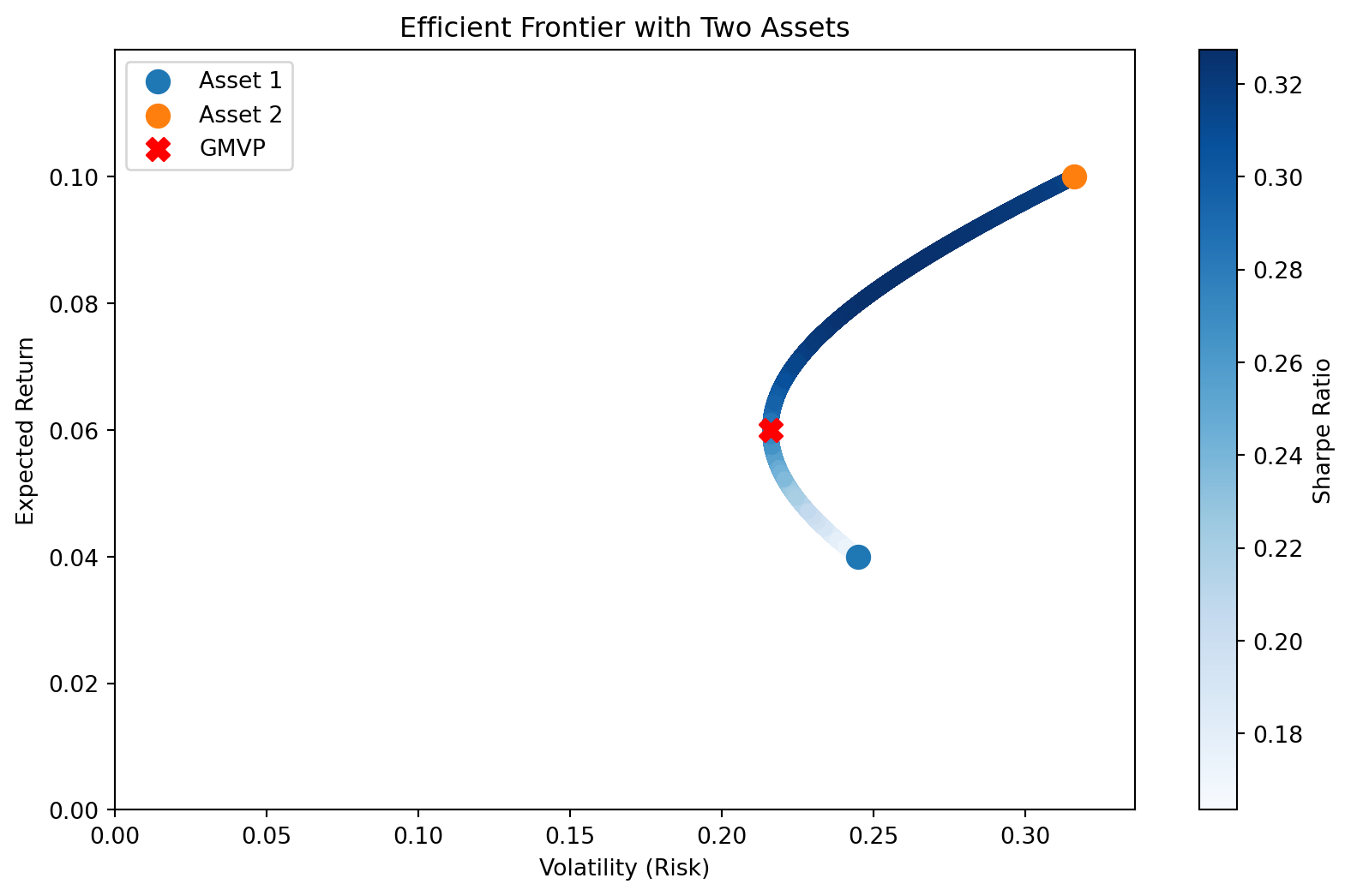
# Plot the efficient frontier
plt.figure(figsize=(10, 6))
plt.scatter(
    results[0, :], results[1, :], c=results[2, :], cmap="Blues", marker="o", alpha=1
)
plt.colorbar(label="Sharpe Ratio")

# Plot individual assets as red dots
plt.scatter(
    individual_volatility[0],
    mean_returns[0],
    # color="red",
    marker="o",
    s=100,
    label="Asset 1",
)
plt.scatter(
    individual_volatility[1],
    mean_returns[1],
    # color="blue",
    marker="o",
    s=100,
    label="Asset 2",
)
# Plot GMVP
plt.scatter(gmvp_volatility, gmvp_return, color="red", marker="X", s=100, label="GMVP")

# Set axis limits to start from 0
plt.xlim(0, np.max(results[0, :]) + 0.02)  # Add a small margin on the right
plt.ylim(0, np.max(results[1, :]) + 0.02)  # Add a small margin on the top

# Annotate the plot
plt.title("Efficient Frontier with Two Assets")
plt.xlabel("Volatility (Risk)")
plt.ylabel("Expected Return")
plt.legend(loc="upper left")
plt.show()
Figure 1: MPT and efficient frontier

Minimum risk portfolio (Global Minimum Variance Portfolio, GMVP)

  • Combination of assets that reduces the variance of portfolio returns on the lowest feasible level.

Moody’s Analytics RiskFrontier Model

Moody’s Analytics RiskFrontier model (previously Portfolio Manager model) estimates the return, risk and correlations between loans in an FI’s loan portfolio (with its own proprietary methods), which are then incorporated into the standard MPT equations to get an estimate of the risk and return of the FI’s loan portfolio.

  1. Moody’s Analytics Credit Monitor model estimates EDF (Expected Default Frequency) to examine the default risk of individual loans.
  2. Moody’s Analytics RiskFrontier model then uses EDF to identify the overall risk of the loan portfolio.
    • Does not require loan returns to be normally distributed
    • Applies MPT to the loan portfolio, although many loans have non-traded aspects

Moody’s Analytics RiskFrontier Model (cont’d)

In Moody’s Analytics RiskFrontier model, portfolio return and risk are a function of:

  • the extent to which loan (exposure) values can change over a one-year horizon, and
    • based on EDF and the loss given default (LGD)
  • how these value changes move together across different loans in the loan portfolio (correlations).
    • based on the joint impact of close to 1,000 different systematic factors, which reflect the global economy, region, industry, and country

Moody’s Analytics RiskFrontier Model (cont’d)

Required input variables:

  1. \(R_i\): Expected return on a loan to a borrower \(i\) is the loan’s all-in-drawn spread (\(AIS\)) minus expected loss (expected default frequency times loss given default (LGD)).1 \[ R_i = AIS_i - E(L_i) = AIS_i - (EDF_i\times LGD_i) \]
    • The Basel Committee assessed a fixed 45% LGD on secured loans if fully secured by physical, non–real estate collateral and 40% if fully secured by receivables.
  1. \(\sigma_i\): Risk of a loan to borrower \(i\), “unexpected loss”, is the volatility of the loan’s default rate \(\sigma_{D_i}\) times the amount lost given default (LGD).2 \[ \sigma_i = UL_i = \sigma_{D_i} \times LGD_i = \sqrt{EDF_i(1-EDF_i)} \times LGD_i \]
    • Assume defaults are binomially distributed (default or not), the standard deviation of default rate (\(\sigma_{D_i}\)) is \(\sqrt{EDF_i(1-EDF_i)}\).
  1. \(\rho_{ij}\): Correlation of default risks between borrowers \(i\) and \(j\) is the correlation between the systematic return components of the asset returns of \(i\) and \(j\).

Moody’s Analytics RiskFrontier Model (cont’d)

To measure the unobservable default risk correlation between any two borrowers, the Moody’s Analytics Global Correlation Model (GCORR) uses the systematic asset return components of the two borrowers and calculates a correlation that is based on a factor model rather than direct historical observations.

Figure 2: GCorr Corporate Factor Structure

Figure 2 provides a visual representation of the Moody’s Analytics GCorr Corporate factor structure.

Moody’s Analytics RiskFrontier Model (example)

Suppose that an FI holds two loans with the following characteristics. Assume that the correlation \(\rho_{12}=-0.25\), what are the return and risk of the portfolio?

Loan \(i\) \(X_i\) Spread between loan rate and FI’s cost of funds Fees LGD EDF
1 0.6 5% 2% 25% 3%
2 0.4 4.5% 1.5% 20% 2%

The return and risk on loan 1 are:

\[ \begin{aligned} R_1 &= (0.05+0.02) - (0.03\times0.25) = 0.0625 \\ \sigma_1 &= \sqrt{0.03\times0.97} \times 0.25 = 0.04265 \end{aligned} \]

The return and risk on loan 2 are:

\[ \begin{aligned} R_2 &= (0.045+0.015) - (0.02\times0.2) = 0.056 \\ \sigma_2 &= \sqrt{0.02\times0.98} \times 0.2 = 0.028 \end{aligned} \]

The return and risk of the portfolio are then:

\[ \begin{aligned} R_p &= 0.6\times 0.0625 + 0.4\times 0.056 = 0.0599 \text{ or } 5.99\% \\ \sigma_p^2 &= (0.6)^2(0.04265)^2 + (0.4)^2(0.028)^2 + 2(0.6)(0.4)(-0.25)(0.04265)(0.028) = 0.0006369 \\ \sigma_p &= \sqrt{0.0006369} = 0.0252 = 2.52\% \end{aligned} \]

Partial application of portfolio theory

  1. Loan volume-based models
  2. Loan loss ratio-based models

Partial application of portfolio theory: Loan volume-based models

Direct application of MPT is often difficult for FIs lacking information on market prices because many of the loans are not always able to be bought and sold in established markets.

Data can be gathered from:

  • Reports to the central bank
  • Data on shared national credit
  • Commercial databases

Data provides market benchmarks against which FIs can compare their loan portfolios.

Table 3: Allocation of the Loan Portfolio to Different Sectors (in percentages)
(1) National (2) Bank A (3) Bank B
Real estate 45% 65% 10%
C&I 30 20 25
Individual 15 10 55
Others 10 5 10
Total 100 100 100

Partial application of portfolio theory: Loan volume-based models (cont’d)

  • Deviations from the market portfolio benchmark indicate the relative degree of loan concentration.
  • Relative measure of loan allocation deviation:

\[ \sigma_j = \sqrt{\frac{\sum_{i=1}^N (X_{ij}-X{i})^2}{N}} \]

where

  • \(\sigma_j\) is the standard deviation of bank \(j\)’s asset allocation proportions from the national benchmark
  • \(X_i\) is the national asset allocations
  • \(X_{ij}\) is the asset allocation proportions of the \(j\)th bank
  • \(N\) is the number of observations or loan categories

Partial application of portfolio theory: Loan volume-based models (cont’d)

Refer to Table 3. We get the deviation of Bank A’s loan portfolio allocation as follows:

\[ \begin{aligned} (X_{1A}-X_1)^2 &= (0.65-0.45)^2 = 0.04 \\ (X_{2A}-X_2)^2 &= (0.20-0.30)^2 = 0.01 \\ (X_{3A}-X_3)^2 &= (0.10-0.15)^2 = 0.0025 \\ (X_{4A}-X_4)^2 &= (0.05-0.10)^2 = 0.0025 \end{aligned} \] and therefore \[ \sigma_A = \sqrt{\frac{0.04+0.01+0.0025+0.0025}{4}} = 11.73\% \]

Partial application of portfolio theory: Loan loss ratio-based models

Estimates systematic loan loss risk of a particular sector or industry to the loan loss risk of an FI’s total loan portfolio

Use of time-series regression of quarterly losses:

\[ \frac{\text{Sectoral losses in the } i\text{th sector}}{\text{Loans to the } i\text{th sector}} = \alpha + \beta \frac{\text{Total loan losses}}{\text{Total loans}} \]

where

  • \(\alpha\) measures the loan loss rate for a sector that has no sensitivity to losses on the aggregate loan portfolio
  • \(\beta\) measures the systematic loss sensitivity of the \(i\)th sector loans to total loan losses

The implication of this model is that sectors with lower \(\beta\)s could have higher concentration limits than high \(\beta\) sectors—since low \(\beta\) loan sector risks (loan losses) are less systematic (that is, are more diversifiable in a portfolio sense).

Regulatory models

  • Federal Reserve’s 1994 Ruling on Credit Concentration Risk:
    • Adopted a subjective approach based on examiner discretion.
    • Rejected technical models due to insufficient data and undeveloped methods at the time.
  • 2006 Regulatory Changes:
    • Bank for International Settlements (BIS): Released guidance on credit risk assessment and valuation for loans, structured around 10 principles on risk assessment and supervisory evaluation.
    • Office of the Comptroller of the Currency (OCC): Released guidance on sound risk management practices for commercial real estate lending.
  • OCC/Fed Joint Study on 2006 CRE Concentration Guidance (April 2013):
    • 13% of banks with construction loans exceeding 100% of capital failed.
    • 23% of banks exceeding both construction and total CRE lending criteria failed, compared to only 0.5% of banks that did not exceed either criterion.
    • Regulators encouraged financial institutions to review their policies and practices related to CRE lending.

Use of derivatives to manage credit risk

Credit derivatives

  • Diversification of loan portfolio helps FIs to manage their credit risk exposure.
  • New types of derivative instruments are now available to better allow FIs to hedge their credit risk both on individual loans or on loan portfolios.
    • Credit forwards, options, and swaps.
  • These credit derivatives allow FIs to separate the credit risk exposure from the lending process itself.

Credit forward contracts and credit risk hedging

A credit forward is a forward agreement that hedges against an increase in default risk on a loan (a decline in credit quality of borrower) after the loan rate is determined and the loan is issued.

  • Common buyers are insurance companies who bears the risk of an increase in default risk on the benchmark bond of the borrower
  • Common sellers are banks
  • Specifies a credit spread on a benchmark bond issued by a borrower
  • Example: BBB bond at time of origination may have 2 per cent spread over US Treasury of same maturity

Credit forward contracts and credit risk hedging (cont’d)

Table 4: Payment pattern on a credit forward contract
Credit Spread at End of Forward Agreement Credit Spread Seller (bank) Credit Spread Buyer (counterparty)
\(\phi_T>\phi_F\) Receives \((\phi_T - \phi_F) \times MD \times A\) Pays \((\phi_T - \phi_F) \times MD \times A\)
\(\phi_T<\phi_F\) Pays \((\phi_F - \phi_T) \times MD \times A\) Receives \((\phi_F - \phi_T) \times MD \times A\)

where

  • \(\phi_F\) is the credit spread on which the credit forward contract is written
  • \(\phi_T\) is the actual credit spread on the bond when the credit forward matures
  • \(MD\) is the modified duration on the benchmark bond
  • \(A\) is the principal amount of the forward agreement

Payout by the bank is capped since \(\phi_T\geq 0\) (credit spread is non-negative).

  • When a bank gives a loan, it is similar to writing a put option
  • When a bank sells a credit forward, the payoff is similar to buying a put option

Credit options

Use of options to hedge credit risk is a relatively new phenomenon. In September 2021, commercial bank holdings of credit options totaled $233 billion, which represented 6.05% of all credit derivatives outstanding.

  • A credit spread call option is a call option whose payoff increases as the (default) risk premium or yield spread on a specified benchmark bond of the borrower increases above some exercise spread.
  • A digital default option is an option that pays a stated amount in the event of a loan default (the extreme case of increased credit risk).

Credit (default) swaps (CDS)

  • Fastest-growing types of swaps. Most important type of credit derivatives.
  • In 2000, commercial banks’ total notional principal for outstanding credit derivatives was $426 billion.
  • By March 2008, this amount had risen to $16.44 trillion, before falling to $13.44 trillion in 2009.
  • By September 2011, the amount increased to $15.66 trillion, of which $15.31 trillion was CDSs.
  • Due to post-GFC regulations, the notional value of credit derivatives held by banks dropped to $3.9 trillion in September 2021, with $3.4 trillion of this amount being CDS contracts.

Why CDS?

  1. Credit risk is still more likely to cause an FI to fail than is either interest rate risk or FX risk.
  2. CDSs allow FIs to maintain long-term customer lending relationships without bearing the full credit risk exposure from those relationships.

Basics of CDS

  • CDS Payments: The buyer makes periodic payments to the seller (quarterly, semi-annually, or annually) until the end of the swap or a credit event (e.g., default) occurs.
  • Settlement: Upon default, settlement involves either physical delivery of bonds (loans) or a cash payment.
    • The protection buyer receives a payment upon the occurrence of a credit event trigger, but the swap “expires worthless” if no trigger occurs.
  • Cheapest-to-Deliver Option: The CDS buyer has the option to deliver the cheapest qualifying bond or loan when a default happens.
  • No requirement that the CDS buyer actually owns the underlying reference securities.
  • The CDS buyer hedges its exposure to default risk, but there is still counterparty credit risk in the event that the seller fails to perform their obligations under the terms of the contract.1

We examine two types of credit swaps:

  1. total return swap
  2. pure credit swap

Credit swaps: total return swaps

A total return swap involves swapping an obligation to pay interest at a specified fixed or floating rate for payments representing the total return on a loan or a bond (interest and principal value changes) of a specified amount.

The figure below illustrates a total return swap.1

Code
graph LR
    A[Other FI]
    B[FI lender]
    B -- Loan --> C[Customer]
    subgraph Total Return Swap
    B -- "$f+{(P_T-P_0)}/{P_0}$" --> A
    A -- 1-year LIBOR --> B
    end

Total Return Swap
Loan
\(f+{(P_T-P_0)}/{P_0}\)
1-year LIBOR
Other FI
FI lender
Customer

The FI lender pays a fixed annual rate \(f\) plus changes in the market value of the loan and receives a variable rate payment (e.g., 1-year LIBOR).

  • Interest rate risk remains

Credit swaps: total return swaps (cont’d)

Code
import numpy as np
import matplotlib.pyplot as plt

np.random.seed(8003)
# Parameters for the TRS
notional = 1_000_000  # Notional amount (1 million)
fixed_rate = 0.03  # Fixed annual rate paid by the TRS receiver (3%)
asset_volatility = 0.1  # Volatility of the asset's return (10%)
years = 5  # Time period of the TRS (5 years)
periods_per_year = 4  # Payments per year (quarterly)


# Generate the timeline for TRS payments
def generate_trs_timeline(
    notional, fixed_rate, asset_volatility, years, periods_per_year=4
):
    # Set up the timeline with quarterly periods
    total_periods = periods_per_year * years
    time_points = np.arange(1, total_periods + 1) / periods_per_year

    # Calculate the periodic fixed payment amount (quarterly)
    periodic_fixed_payment = (
        -notional * fixed_rate / periods_per_year
    )  # Fixed payment made by TRS receiver

    # Simulate random returns on the asset
    asset_returns = np.random.normal(loc=0, scale=asset_volatility, size=total_periods)

    # Initialize lists to store the results
    total_returns = np.zeros(total_periods)
    payments = np.zeros(total_periods)

    for period in range(total_periods):
        # Total return on the asset (positive or negative)
        total_return = notional * asset_returns[period]
        total_returns[period] = total_return

        # Net payment for the TRS receiver (positive if receiving total return, minus fixed payment)
        payments[period] = total_return + periodic_fixed_payment

    return time_points, payments, total_returns


# Simulate TRS payments with different asset volatilities
volatilities = [0.05]  # Different volatilities to simulate
simulations = {}

for vol in volatilities:
    timeline, payments, total_returns = generate_trs_timeline(
        notional, fixed_rate, vol, years, periods_per_year
    )
    simulations[vol] = payments

# Plot the timelines as bar charts
plt.figure(figsize=(12, 8))
bar_width = 0.2  # Width of each bar

# Generate bar charts for each volatility
for idx, (vol, payments) in enumerate(simulations.items()):
    plt.bar(
        timeline + idx * bar_width * 0.1,
        payments,
        width=bar_width,
        color="#A6192E",
        label=f"Volatility: {vol*100:.0f}%",
    )

# Customize the plot
plt.title(f"{years}-Year Total Return Swap Payments Example")
plt.xlabel("Time (Years)")
plt.ylabel("Net Payment Amount ($)")
plt.axhline(0, color="black", linewidth=1)
plt.grid(True)
plt.legend()

# Show the plot
plt.show()
Figure 3: Total Return Swap Payments Example

Credit swaps: pure credit swaps

Interest-rate sensitive element stripped out leaving only the credit risk.

Similar to buying an insurance:

  • If default, the counterparty makes the default payment
  • If not default, the FI receives nothing from the counterparty.
Code
graph LR
    A[Other FI]
    B[FI lender]
    B -- Loan --> C[Customer]
    subgraph Pure Credit Swap
    B -- Fee --> A
    A -. Default payment .-> B
    end

Pure Credit Swap
Loan
Fee
Default payment
Other FI
FI lender
Customer

Credit swaps: pure credit swaps (cont’d)

Code
import numpy as np
import matplotlib.pyplot as plt

np.random.seed(8003)
# Parameters for the CDS
notional = 1_000_000  # Notional amount (1 million)
cds_spread = 0.02  # Annual CDS spread (2%)
recovery_rate = 0.9  # Recovery rate in case of default (10%)
years = 5  # Time period of the CDS (5 years)
periods_per_year = 4  # Payments per year (quarterly)


# Generate the timeline for CDS payments
def generate_cds_timeline(
    notional, cds_spread, default_probability, recovery_rate, years, periods_per_year=4
):
    # Set up the timeline with quarterly periods
    total_periods = periods_per_year * years
    time_points = np.arange(1, total_periods + 1) / periods_per_year

    # Calculate the periodic payment amount (quarterly)
    periodic_payment = (
        -notional * cds_spread / periods_per_year
    )  # Negative for payments

    # Initialize lists to store the results
    payments = np.zeros(total_periods)

    # Simulate payments and default events
    for period in range(total_periods):
        if np.random.rand() < default_probability / periods_per_year:
            # Default occurs at this period
            default_loss = notional * (
                1 - recovery_rate
            )  # Positive for the payment received on default
            payments[period] = default_loss
            payments[period + 1 :] = 0  # No more payments after default
            break
        else:
            # Regular payment
            payments[period] = periodic_payment

    return time_points, payments


# Simulate multiple series with different default probabilities
default_probabilities = [0.02, 0.1]  # Different default probabilities
colors = ["#D6D2C4", "#A6192E"]

simulations = {}

# Generate timelines for each default probability
for prob in default_probabilities:
    timeline, payments = generate_cds_timeline(
        notional, cds_spread, prob, recovery_rate, years, periods_per_year
    )
    simulations[prob] = payments

# Plot the timelines as bar charts
plt.figure(figsize=(12, 8))
bar_width = 0.2  # Width of each bar

# Generate bar charts for each probability
for idx, (prob, payments) in enumerate(simulations.items()):
    plt.bar(
        timeline + idx * bar_width * 0.1,
        payments,
        width=bar_width,
        color=colors[idx],
        label=f"Default Probability: {prob*100:.0f}%",
    )

plt.title(f"{years}-Year Pure CDS Payments Example")
plt.xlabel("Time (Years)")
plt.ylabel("Payment Amount ($)")
plt.axhline(0, color="black", linewidth=1)
plt.grid(True)
plt.legend()
plt.show()
Figure 4: Pure CDS Payments Example

Finally…

Suggested readings

References

Saunders, Anthony, Marcia Millon Cornett, and Otgo Erhemjamts. 2023. Financial Institutions Management ISE. 11th ed. McGraw Hill.