AFIN8003 Week 11 - Sovereign Risk, Foreign Exchange Risk, and Off-Balance-Sheet Risk

Banking and Financial Intermediation

Dr. Mingze Gao

Department of Applied Finance

2024-10-16

Sovereign Risk, Foreign Exchange Risk, and Off-Balance-Sheet Risk

Introduction

• Foreign Exchange Risk: Also known as currency risk, this is the potential for losses due to changes in exchange rates. It affects businesses and financial institutions involved in cross-border transactions, as fluctuations can alter the value of foreign-denominated assets, liabilities, or revenues.

• Sovereign Risk: This risk arises when a government defaults on its debt or restricts its residents from fulfilling international debt obligations. It reflects the political and economic stability of a country, impacting investors and financial institutions with exposure to that country’s assets.

• Off-Balance-Sheet Risk: These are risks associated with contingent liabilities or commitments that do not appear on the balance sheet. Common examples include guarantees, derivatives, and letters of credit, which can lead to substantial losses if the underlying exposures materialize.

Foreign exchange risk

Foreign exchange rates

A foreign exchange (FX) rate is the price at which one currency (e.g., the U.S. dollar) can be exchanged for another currency (e.g., the Australian dollar).

Two basic types of FX transactions:

1. Spot FX transactions involve the immediate settlement, or exchange, of currencies at the current (spot) exchange rate.
2. Forward FX transactions involve the exchange of currencies at a specified exchange rate (i.e., the forward exchange rate) which is settled at some specified date in the future.

Source of FX risk exposure

Assets and liabilities denominated in foreign currencies

• making foreign currency loans
• issuing foreign currency-denominated debt

The trading of foreign currencies involves

• purchase and sale of currencies to complete international transactions
• facilitating positions in foreign real and financial investments
• accommodating hedging activities
• speculation

Substantial risk arises via open positions (unhedged positions).

FX exposure

An FI’s overall FX exposure in any given currency can be measured by the net position exposure, which is measured in local currency as

\[ \begin{aligned} \text{Net exposure}_i &= (\text{FX assets}_i - \text{FX liabilities}_i) + (\text{FX bought}_i - \text{FX sold}_i) \\ &=\text{Net foreign assets}_i + \text{Net FX bought}_i \end{aligned} \]

where \(i\) represents the \(i\)th currency.

FI could match its foreign currency assets to its liabilities in a given currency and match buys and sells in its trading book in that foreign currency

• reduce its foreign exchange net exposure to zero and thus avoid FX risk.

Financial holding companies can aggregate their foreign exchange exposure through their banking, insurance and funds management businesses under one umbrella

• allows them to reduce their net foreign exchange exposure across all units.

FX rate volatility and FX exposure

We can measure the potential size of an FI’s FX exposure as:

\[ \begin{aligned} \text{Dollar loss/gains in currency } i &= \text{Net exposure in foreign currency } i \text{ measured in local currency} \\ &\times \text{Shock (volatility) to the exchange rate of local currency to foreign currency } i \end{aligned} \]

• Greater exposure to a foreign currency combined with greater volatility of the foreign currency implies greater daily earnings at risk (DEAR).
• Reason for FX volatility: fluctuations in the demand for and supply of a country’s currency

FX rate volatility and FX exposure (cont’d)

\[ \begin{aligned} \text{Dollar loss/gains in currency } i &= \text{Net exposure in foreign currency } i \text{ measured in local currency} \\ &\times \text{Shock (volatility) to the exchange rate of local currency to foreign currency } i \end{aligned} \]

Example

On September 8, 2024, an Australian FI has a net exposure to New Zealand dollar (NZD) of NZD$1,000,000. The exchange rate of AUD to NZD was 1.08 AUD/NZD.

It is now October 8, 2024, and the exchange rate becomes 1.10 AUD/NZD. The AUD has depreciated in value relative to the NZD. Calculate the FI’s dollar loss/gain for this shock to the AUD/NZD exchange rate.

• The AUD value of the NZD position on September 8 is \(\$1,000,000\times 1.08=\$1,080,000\).
• The AUD value of the NZD position on October 8 is \(\$1,000,000\times 1.10=\$1,100,000\).
• The gain from the net long position in NZD is \(\$1,100,000-\$1,080,000=\$20,000\).

Or, the dollar loss/gain is

\(\text{NZD}\$1,000,000 \times (1.10 - 1.08) = \text{AUD}\$20,000\).

FX rate volatility and FX exposure (cont’d)

The FI has a €2.0 million long trading position in spot euros at the close of business on a particular day. The exchange rate is €0.80/$1, or $1.25/€, at the daily close. Looking back at the daily changes in the exchange rate of the euro to dollars for the past year, the FI finds that the volatility or standard deviation (\(\sigma\)) of the spot exchange rate was 50 basis points (bp). What is the DEAR?

\[ \text{DEAR} = \text{Dollar value of position} \times \text{FX volatility} \]

• Dollar value of position = €2.0 x 1.25 $/€ = $2.5 million
• FX volatility = 2.33\(\sigma\) = 2.33 x 0.005 = 0.01165
• DEAR = $2,500,000 x 0.01165 = $29,125

Interaction of interest rate, inflation, and exchange rates

• Global financial markets are increasingly interconnected, so are interest rates, inflation, and foreign exchange rates.
• We now explore how inflation in one country affects its foreign currency exchange rates, focusing on purchasing power parity (PPP).
• Next, we examine the relationship between domestic/foreign interest rates and spot/forward foreign exchange rates, known as interest rate parity (IRP).

Purchasing Power Parity

Nominal interest rate \(R\) is basically the sum of inflation \(i\) and real interest rate \(r\):

For two countries, e.g., Australia (AU) and United States (US), we have:

\[ \begin{aligned} R_{AU} &= i_{AU} + r_{AU} \\ R_{US} &= i_{US} + r_{US} \end{aligned} \]

Assuming real interest rates are equal across countries: \(r_{AU}=r_{US}\), then

\[ R_{AU} - R_{US} = i_{AU} - i_{US} \]

That is, the (nominal) interest rate spread between Australia and the United States represents the difference in inflation rates between the two countries.

Important

When inflation rates and/or interest rates change, foreign exchange rates (without government control) should adjust to account for relative differences in the price levels (inflation) between the two countries.

The Purchasing Power Parity (PPP) is one theory explaining how this adjustment takes place.

Purchasing Power Parity (cont’d)

Let’s think of an example to illustrate the idea of PPP.

• Imagine you have $1 and can buy one candy in the U.S. Now, let’s say in Japan, 100 yen also buys one candy.
• If $1 is worth 100 yen, things are “balanced”.
• But if candy’s price in Japan increases to 150 yen (inflation in Japan), your $1 won’t buy as much candy anymore.

PPP states that, in different countries, the same money should buy the same amount of goods and services. So, when prices change, the money’s value changes, too, to keep things fair.

• The relative value of money is the exchange rate!

Purchasing Power Parity (cont’d)

Tip

The PPP says that the most important factor determining exchange rates is the price differences drive trade flows and thus demand for and supplies of currencies.

Specifically, the PPP theorem states that the change in the exchange rate between two countries’ currencies is proportional to the difference in the inflation rates in the two countries. That is:

\[ i_{domestic} - i_{foreign} = \frac{\Delta S_{domestic/foreign}}{S_{domestic/foreign}} \]

where

• \(S_{domestic/foreign}\) is the spot exchange rate of the domestic currency for the foreign currency
• \(\Delta S_{domestic/foreign}\) is the change in the one-period spot exchange rate

Purchasing Power Parity (cont’d)

Suppose that the current spot exchange rate of Australian dollars for Chinese yuan, \(S_{AUD/CNY}\), is 0.17 (i.e. 0.17 dollars, or 17 cents is equal to 1 yuan). The price of Chinese-produced goods increases by 10 per cent (i.e. inflation in China \(i_C\), is 10 per cent), and the Australian price index increases by 4 per cent (i.e. inflation in Australia, \(i_{AUS}\), is 4 per cent). What will be the change of the exchange rate?

According to PPP:

\[ i_{AUS} - i_{C} = \frac{\Delta S_{AUD/CNY}}{S_{AUD/CNY}} \]

So that

\[ 0.04 - 0.1 = \frac{\Delta S_{AUD/CNY}}{0.17} \]

Solving the equation, we get \(\Delta S_{AUD/CNY} = −0.0102\). Thus, it costs 1.02 cents less to receive a yuan. The Chinese yuan depreciates in value by 6 per cent against the Australian dollar as a result of its higher relative inflation rate. In other words, a 6 per cent fall in the yuan’s value translates into a new exchange rate of 0.1598 dollars per yuan.

Purchasing Power Parity (cont’d)

The theory behind purchasing power parity is the law of one price, an economic concept which states that in an efficient market, if countries produce a good or service that is identical to that in other countries, that good or service must have a single price, no matter where it is purchased.

Interest Rate Parity

To illustrate (covered) interest rate parity (IRP), let’s consider two investment strategies.

Strategy 1: Domestic Investment

• You invest $1 domestically at an interest rate \(r_d\) for one period.
• After one period, your investment grows to \(1 + r_d\).

Strategy 2: Foreign Investment with Forward Contract

• You convert $1 into foreign currency at the current spot exchange rate \(S\), which gives \(1/S\) foreign currency.
• You then invest the foreign currency amount in a foreign asset at the interest rate \(r_f\) for one period.
• After one period, this investment grows to \((1 + r_f)\).
• You lock in the forward exchange rate \(F\) now to convert the foreign currency back to domestic currency after one period.

For these two strategies to have the same return (and eliminate arbitrage opportunities), the returns on both should be equivalent when the foreign investment is converted back using the forward rate. This gives us the CIRP condition:

\[ 1 + r_d = \frac{(1 + r_f) \cdot F}{S} \]

Rearranging, we can see the relation between interest rates and the forward rate:

\[ F = S \cdot \frac{1 + r_d}{1 + r_f} \]

Interest Rate Parity (cont’d)

Assume the interest rate on Australian dollar securities at time \(t\) equals 5 per cent and the interest rate on euro loans at time \(t\) is 10 per cent. Further, suppose the $/€ spot exchange rate (\(S_t\)) at time t is $0.60/€1 and the future exchange rate (\(F_t\)) is $0.55/€1. If the spot exchange rate rises to $0.65/€1, what is the change on the forward exchange rate?

To find the change in the forward exchange rate due to a change in the spot exchange rate, we can start by using the IRP condition:

\[ F_t = S_t \cdot \frac{1 + r_d}{1 + r_f} \]

• Domestic interest rate (Australia), \(r_d = 5\% = 0.05\)
• Foreign interest rate (Euro), \(r_f = 10\% = 0.10\)
• Initial spot exchange rate, \(S_t = 0.60\) AUD/EUR
• Initial forward exchange rate, \(F_t = 0.55\) AUD/EUR
• New spot exchange rate, \(S'_t = 0.65\) AUD/EUR

Let’s calculate the new forward rate using CIRP, then we’ll find the change in the forward rate.

Step 1: Calculate the New Forward Rate \(F'_t\)

\[ \begin{aligned} F'_t &= S'_t \cdot \frac{1 + r_d}{1 + r_f} \\ &= 0.65 \cdot \frac{1 + 0.05}{1 + 0.10} \\ &\approx 0.6205 \text{ AUD/EUR} \end{aligned} \]

Step 2: Calculate the Change in the Forward Rate

Now, find the change between the new forward rate and the initial forward rate:

\[ \begin{aligned} \Delta F_t &= F'_t - F_t \\ &= 0.6205 - 0.55 \\ &\approx 0.0705 \text{ AUD/EUR} \end{aligned} \]

The forward exchange rate increases by approximately 0.0704 AUD/EUR as a result of the rise in the spot exchange rate.

Managing FX risk

On-balance-sheet hedging

• Requires duration matching to control exposure to foreign interest rate risk
• A direct match of foreign assets and liabilities can result in positive profits for the FI

Off-balance-sheet hedging

• Uses forwards, futures, options and swaps
• Example: hedging with forwards allows FI to offset uncertainty regarding the future spot rate on a currency

Sovereign risk

Introduction to sovereign risk

• Mismatches in the size and maturities of foreign assets and liabilities expose FIs to FX risk.
• Beyond FX risk, holding assets in a foreign country also exposes FIs to country or sovereign risk.
  • e.g., when the foreign corporation may be unable to repay the principal or interest on a loan even if it would like to.
  • the government of the country in which a borrower is headquartered may prohibit or limit debt payments
    • foreign currency shortages, adverse political reasons, and more.

Credit risk vs sovereign risk

• Credit Risk: This is the risk that a borrower (like a domestic firm) might refuse or be unable to repay its debt. If this happens, lenders can negotiate loan restructuring or, ultimately, pursue bankruptcy proceedings to recover assets. This type of risk is typically manageable through legal proceedings within the borrower’s own country.

• Sovereign Risk: This arises when a government (such as the Greek government) intervenes, restricting a domestic corporation from repaying its foreign debts, regardless of the corporation’s financial health. Unlike credit risk, sovereign risk is largely out of the borrower’s control and independent of the borrower’s creditworthiness. In cases of sovereign risk, international lenders have limited legal options, as there’s no global court to enforce debt repayment or asset liquidation against a sovereign state.

Therefore, lending decisions to parties in foreign countries require two steps:

1. credit quality assessment of borrower
2. sovereign risk quality assessment of country

Forms of sovereign risk

A sovereign country’s (negative) decisions on its debt obligations or the obligations of its public and private organizations may take two forms: repudiation and restructuring.

1. Debt repudiation
   • An outright cancellation of all a borrower’s current and future foreign debt and equity obligations
   • In 1996, World Bank, IMF and major governments around the world forgave the debt of the world’s poorest, most heavily indebted countries (HIPCs)
   • By 2021, 36 countries had received debt relief under the HIPC initiative, 30 of them in Africa, which totaled a reduction of $76 billion on their outstanding debt
2. Debt restructuring
   • Change the contractual terms of a loan, such as maturity and interest payment
     • Delay the payment
     • Pay less interest
   • Most common form of sovereign risk

Repudiation vs restructuring

Repudiation was more common before World War II, while post World War II, restructuring is more likely.

• One reason is that most postwar international debt has been bank loans, while before the war it was mostly foreign bonds.
• Bondholders are diverse - hard to reach an agreement to changes in the contractual terms on a bond.
• Fewer FIs involved in international lending syndicates.
• Many international loan contracts contain “cross-default” provisions: one loan default automatically triggers all loans’ default to prevent a country from selectively defaulting.
• Bank bailouts for large banks create (mis)incentives.

Country risk evaluation

An FI can rely on both outside evaluation services or develop its internal evaluation models for sovereign risk.

• Outside Evaluation Models
  • The Euromoney Country Risk Index
  • The Institutional Investor Credit Ratings
  • OECD Country Risk Classifications
• Internal Evaluation Models
  • Statistical models

Statistical models for country risk evaluation

Most common form of country risk assessment scoring models based on economical factors

1. pick a set of variables that may be important in explaining restructuring probabilities
2. develop the scoring model

Commonly used economic ratios:

1. Total debt service ratio (TDSR)

\[ \begin{aligned} TDSR &= \frac{\text{Total debt service}}{\text{Exports}} \\ &= \frac{\text{Interest} + \text{amortisation on debt}}{\text{Exports}} \\ \end{aligned} \]

A country’s exports are its primary way of generating dollars and other currencies.

• The higher the ratio, the higher sovereign risk.

Note

Check data at World Bank’s DataBank.

Statistical models for country risk evaluation (cont’d)

2. Import ratio (IR)

\[ IR = \frac{\text{Total imports}}{\text{Total FX reserves}} \]

Imports to meet demands - sometimes even food is a vital import - requires FX reserves.

• The higher the ratio, the higher sovereign risk.

Note

In 2020, Greece’s IR was 626% while China’s IR aws 70%. Greece imported more goods and services than it had serves to pay for them.

Statistical models for country risk evaluation (cont’d)

3. Investment ratio (INVR)

\[ INVR = \frac{\text{Real investment}}{\text{GDP}} \]

• The higher the ratio, the lower sovereign risk (arguable).

Statistical models for country risk evaluation (cont’d)

4. Variance of export revenue (VAREX)

\[ VAREX = \sigma^2_{ER} \]

• The higher the variance, the higher sovereign risk.

Statistical models for country risk evaluation (cont’d)

5. Domestic money supply growth (MG)

\[ MG = \frac{\Delta M}{M} \]

• Weaken local currency by pushing up inflation rate.
• The higher the growth, the higher sovereign risk.

Statistical models for country risk evaluation (cont’d)

Develop a scoring model \(f\) as a function of the chosen economic variables:

\[ p = f(TDSR, IR, INVR, VAREX, MG, \dots) \]

where \(p\) can be the probability of restructuring.

Off-balance-sheet risk

Off-balance-sheet (OBS) activities

OBS items are “off-balance-sheet” as they appear frequently as footnotes to financial statements.

In economics terms, OBS items are contingent assets and liabilities that affect the future shape of an FI’s balance sheet. They potentially can produce positive or negative future cash flows for an FI.

• The true picture of net worth should include market value of on- and off-balance-sheet activities.

Incentives to increase OBS activities:

• Generate additional income
• Avoid regulatory costs or taxes
  • Reserve requirements
  • Deposit insurance premiums
  • Capital adequacy requirements

Major types of OBS activities

• Loan commitment: Contractual commitment to make a loan up to a stated amount at a given interest rate in the future.
• Letters of credit: Contingent guarantees sold by an FI to underwrite the performance of the buyer of the guaranty.
• Derivative contract: Agreement between two parties to exchange a standard quantity of an asset at a predetermined price at a specified date in the future.
• When-issued trading: Trading in securities prior to their actual issue.
• Loans sold: Loans originated by an FI and then sold to other investors that (in some cases) can be returned to the originating institution in the future if the credit quality of the loans deteriorates.

Loan commitments

• Commitment to make a loan up to a stated amount at a given interest rate in the future
• Nowadays very popular, sometimes more so than spot loans
• Charge up-front fee and back-end fee

The upfront fee applies on the whole commitment size and the back-end fee applies on any unused balances at the end of the period.

Example of the fees

Suppose an FI gives an one-year $10 million loan commitment to a firm with an upfront fee of 1/8% and back-end fee of 1/4%.

The upfront fee is \(\$10,000,000 \times 1/8\% = \$12,500\).

If the firm takes down only $8 million over the year, the back-end fee is \(\$10,000,000\times 1/4\% = \$5,000\).

Loan commitments (cont’d)

For a one-year loan commitment, let:

• Base rate \(BR=12\%\)
• Risk premium \(\phi=2\%\)
• Upfront fee \(f_1=1/8\%\)
• Back-end fee \(f_2=1/4\%\)
• Compensating balance \(b=10\%\)
• Reserve requirements \(RR=10\%\)
• Average takedown rate \(td=75\%\)

Then, the promised return \(1+k\) of the loan commitment is

\[ \begin{aligned} 1+k &= 1+ \frac{f_1+f_2(1-td) + (BR+\phi) td}{td - b\times td (1-RR)} \\ &= 1+ \frac{0.00125+0.0025(1-0.75) + (0.12+0.02) 0.75}{0.75 - 0.1\times 0.75 (1-0.1)} \\ &= 1.1566 \end{aligned} \]

So \(k=15.66\%\).

Risks associated with loan commitments

• Interest rate risk
  • On fixed-rate loan commitments the bank is exposed to interest rate risk
  • On floating-rate commitments, there is still exposure to basis risk
• Draw-down risk
  • Uncertainty of timing of draw-downs exposes bank to risk
  • Back-end fees are intended to reduce this risk
• Credit risk
  • Credit rating of the borrower may deteriorate over the life of the commitment
  • Addressed through ‘adverse material change in conditions’ clause
• Aggregate funding risk
  • During a credit crunch, bank may find it difficult to meet all of the commitments (compare to externality effect)
  • Bank may need to adjust its risk profile on the balance sheet in order to guard against future draw-downs on loan commitments

Letter of credit

1. Documentary (Commercial) letters of credit (LCs)
   • Contingent guarantees to underwrite the trade or commercial performance
   • Widely used in both domestic and international trade

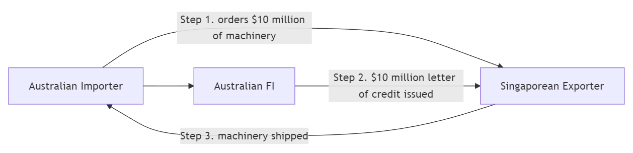
Commercial LC

2. Standby letters of credit (SLCs)
   • Cover contingencies potentially more severe and less predictable than those covered by LCs

Risks associated with letters of credit

The buyer of the LC may fail to perform as promised under the contractual obligation

• During the GFC, many US firms were unable to pay their maturing commercial paper (CP) obligations in the US. The amount of potential defaults would have crippled already liquidity-strapped FIs that had written standby letters of credit backing the CP issues.
• In response, the US Federal Reserve Board (central bank) announced a support mechanism for the CP market to provide liquidity to short-term funding markets, through which the Federal Reserve purchased CPs.
• Thus rather than having to draw on FI letters of credit to pay the CP liabilities, the US government bailed out these securities and the FIs that were backing them.

Derivative contract

• FIs can be either
  • users of derivative contracts for hedging and other purposes, or
  • dealers that act as counterparties in trades with customers for a fee
• In Australia, most banks act in both capacities
• Futures, forwards, swaps and options
  • Forward contracts involve substantial counterparty risk
  • Other derivatives create far less default risk
  • Market risk

Sale of when-issued securities

• Commitments to buy and sell securities before they are issued: ‘when issued (WI) trading’
• Example: new issue of T-Notes announced by RBA
• Banks who bid in the T-Notes auction can trade them before the announcement of the successful bidders through forward sales.
• FIs may sell the yet-to-be-issued Treasury securities for forward delivery to customers in the secondary market at a margin above the price they expect to pay at the tender.
• Risk of ‘over-commitment’

Loans sold

• FI originates loans and sells them to outside investors
• Potential outside investors
  • Other banks
  • Insurance companies
  • Unit trusts
  • Corporations
• Loans sold are an indication of FIs moving from asset-transformers to brokers
• Recourse:the ability to put an asset or loan back to the seller should the credit quality of that asset deteriorate
  • ‘No recourse’: loan buyer bears all default risk if loan goes bad
  • With recourse: long-term contingent credit risk for loan seller

Role of OBS activities in reducing risk

• OBS activities are not always risk-increasing activities
• In many cases they are hedging activities designed to mitigate exposure to interest rate risk, foreign exchange risk etc.
• OBS activities can decrease an FI’s insolvency risk
• OBS activities are frequently a source of fee income, especially for the largest, most credit-worthy banks

Finally…

Suggested readings

References